PDF

Electric Shielding
Introduction
This is a tutorial application that shows how to model isolated highly conductive objects in the Electric Currents interface. The analysis includes the current terminal and electric shielding boundary conditions.
Model Definition
The modeling domain is a seawater filled box containing an electrode. The sides of the box are insulated while the top has an assigned electric potential of 1 V and the bottom is set to ground.
Boundary Conditions on the Electrode
The first version of the application uses the terminal boundary condition with a zero net current. The electrode then assumes a constant potential determined by the surrounding field. This condition, also known as a floating potential condition, can be a good approximation if the electrode is a much better conductor than the surrounding medium. It can also be used for metal surfaces in electrostatics, where the zero current condition is replaced by a zero total charge.
The second version uses an electric shielding condition instead of the terminal boundary condition. The electric shielding condition requires the specification of the material constituting the thin layer and its thickness. When used for describing thin sheets of conducting materials, the electric shielding condition results in a potential that is assumed to be constant across the depth of the material, but varies on its surface.
Results and Discussion
Figure 1 shows the potential distribution when using the electric shielding condition. The electrode is modeled as a 1 mm thick sheet of titanium bent to form three quarters of a cylinder. The cylinder has a radius of 0.2 m and is centered in a cube with a 1 m side. The result, as seen in the surface plot, is a potential that varies between 0.472 V and 0.476 V on the conductor.
Figure 1: The electric potential distribution on the conductor and in the water when using the electric shielding condition.
For a comparison, with the zero current terminal condition, the potential on the conductor evaluates to a constant 0.474 V.
Application Library path: ACDC_Module/Resistive_Devices/electric_shielding
Modeling Instructions
From the File menu, choose New.
New
In the New window, click  Model Wizard.
Model Wizard
1
In the Model Wizard window, click  3D.
2
In the Select Physics tree, select AC/DC>Electric Fields and Currents>Electric Currents (ec).
3
Click Add.
4
Click  Study.
5
In the Select Study tree, select General Studies>Stationary.
6
Geometry 1
Create the model geometry, starting with the electrode.
Cylinder 1 (cyl1)
1
In the Geometry toolbar, click  Cylinder.
2
In the Settings window for Cylinder, locate the Object Type section.
3
From the Type list, choose Surface.
4
Locate the Size and Shape section. In the Radius text field, type 0.2.
5
In the Height text field, type 0.2.
6
Locate the Position section. In the x text field, type 0.4.
7
In the y text field, type 0.5.
8
In the z text field, type 0.5.
9
Locate the Axis section. From the Axis type list, choose Cartesian.
10
In the x text field, type 1.
11
In the z text field, type 0.
12
Click  Build Selected.
Next, delete the segment of the cylinder that lies in the octant y 0, z0.
Delete Entities 1 (del1)
1
In the Model Builder window, right-click Geometry 1 and choose Delete Entities.
2
3
In the Settings window for Delete Entities, click  Build Selected.
In order to facilitate applying materials and boundary conditions, create a selection of the electrode object.
Electrode
1
In the Geometry toolbar, click  Selections and choose Explicit Selection.
2
In the Settings window for Explicit Selection, locate the Entities to Select section.
3
From the Geometric entity level list, choose Boundary.
4
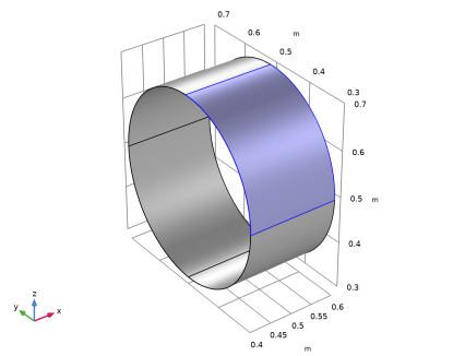
In the Graphics window, click on the three boundaries constituting the electrode.
5
Right-click Explicit Selection 1 (sel1) and choose Rename.
6
In the Rename Explicit Selection dialog box, type Electrode in the New label text field.
7
Finish the geometry by adding a block for the salt-water domain surrounding the electrode.
Block 1 (blk1)
1
In the Geometry toolbar, click  Block.
2
In the Settings window for Block, click  Build All Objects.
3
Click the  Zoom Extents button in the Graphics toolbar.
4
Click the  Wireframe Rendering button in the Graphics toolbar.
Materials
Having created the geometry, proceed to assign materials.
Add Material
1
In the Home toolbar, click  Add Material to open the Add Material window.
2
Go to the Add Material window.
3
In the tree, select Built-in>Titanium beta-21S.
4
Click Add to Component in the window toolbar.
5
In the Home toolbar, click  Add Material to close the Add Material window.
Materials
Titanium beta-21S (mat1)
1
In the Settings window for Material, locate the Geometric Entity Selection section.
2
From the Geometric entity level list, choose Boundary.
3
From the Selection list, choose Electrode.
Sea Water
1
In the Model Builder window, right-click Materials and choose Blank Material.
2
Right-click Material 2 (mat2) and choose Rename.
3
In the Rename Material dialog box, type Sea Water in the New label text field.
4
5
6
In the Settings window for Material, locate the Material Contents section.
7
Electric Currents (ec)
Ground 1
1
In the Model Builder window, under Component 1 (comp1) right-click Electric Currents (ec) and choose Ground.
2
Electric Potential 1
1
In the Physics toolbar, click  Boundaries and choose Electric Potential.
2
3
In the Settings window for Electric Potential, locate the Electric Potential section.
4
In the V0 text field, type 1.
Terminal 1
1
In the Physics toolbar, click  Boundaries and choose Terminal.
2
In the Settings window for Terminal, locate the Boundary Selection section.
3
From the Selection list, choose Electrode.
Next, apply an Electric Shielding node to the electrode for use in the second study. To prevent it from overriding the Terminal node just added, it will be excluded in the first study.
Electric Shielding 1
1
In the Physics toolbar, click  Boundaries and choose Electric Shielding.
2
In the Settings window for Electric Shielding, locate the Boundary Selection section.
3
From the Selection list, choose Electrode.
4
Locate the Thickness section. In the ds text field, type 1[mm].
Mesh 1
Free Tetrahedral 1
In the Mesh toolbar, click  Free Tetrahedral.
Size
1
In the Model Builder window, click Size.
2
In the Settings window for Size, locate the Element Size section.
3
From the Predefined list, choose Fine.
4
Click  Build All.
Study 1
Before solving, disable the Electric Shielding node.
Step 1: Stationary
1
In the Model Builder window, under Study 1 click Step 1: Stationary.
2
In the Settings window for Stationary, locate the Physics and Variables Selection section.
3
Select the Modify model configuration for study step check box.
4
In the tree, select Component 1 (Comp1)>Electric Currents (Ec)>Electric Shielding 1.
5
Click  Disable.
6
In the tree, select Component 1 (Comp1).
7
In the Model Builder window, click Study 1.
8
In the Settings window for Study, locate the Study Settings section.
9
Clear the Generate default plots check box.
This setting is useful if you want full control over which plot groups to create.
10
In the Home toolbar, click  Compute.
Results
Before adding a 3D Plot Group to use for reproducing the plot in Figure 1, add a selection to the solution dataset to hide the block obstructing the view of the electrode.
1
In the Model Builder window, expand the Results node.
Study 1/Solution 1 (sol1)
In the Model Builder window, expand the Results>Datasets node, then click Study 1/Solution 1 (sol1).
Selection
1
In the Results toolbar, click  Attributes and choose Selection.
2
In the Settings window for Selection, locate the Geometric Entity Selection section.
3
From the Geometric entity level list, choose Boundary.
4
From the Selection list, choose Electrode.
Now create the plot.
3D Plot Group 1
1
In the Results toolbar, click  3D Plot Group.
Change some settings in the color legends to better visualize the small variations in electric potential on the surface.
2
In the Settings window for 3D Plot Group, locate the Color Legend section.
3
Select the Show maximum and minimum values check box.
4
Click to expand the Number Format section. Select the Manual color legend settings check box.
5
In the Precision text field, type 4.
Slice 1
1
Right-click 3D Plot Group 1 and choose Slice.
2
In the Settings window for Slice, locate the Plane Data section.
3
In the Planes text field, type 1.
Surface 1
1
In the Model Builder window, right-click 3D Plot Group 1 and choose Surface.
2
In the Settings window for Surface, locate the Coloring and Style section.
3
From the Color table list, choose GrayScale.
Note that the potential on the surface is constant.
3D Plot Group 1
1
In the Model Builder window, click 3D Plot Group 1.
2
In the 3D Plot Group 1 toolbar, click  Plot.
This concludes the work on the terminal version of this application. Next, investigate how the results change as you introduce a finite conductivity and thickness to the plate. Add a separate study for this analysis.
Add Study
1
In the Home toolbar, click  Add Study to open the Add Study window.
2
Go to the Add Study window.
3
Find the Studies subsection. In the Select Study tree, select General Studies>Stationary.
4
Click Add Study in the window toolbar.
5
In the Home toolbar, click  Add Study to close the Add Study window.
Study 2
Step 1: Stationary
Disable the Terminal node for this study, even though this is not strictly necessary as this node is overridden by the Electric Shielding node.
1
In the Settings window for Stationary, locate the Physics and Variables Selection section.
2
Select the Modify model configuration for study step check box.
3
In the tree, select Component 1 (Comp1)>Electric Currents (Ec)>Terminal 1.
4
Click  Disable.
5
In the tree, select Component 1 (Comp1).
6
In the Model Builder window, click Study 2.
7
In the Settings window for Study, locate the Study Settings section.
8
Clear the Generate default plots check box.
9
In the Home toolbar, click  Compute.
Results
Add a selection, restricting this solution dataset to the electrode as well.
Study 2/Solution 2 (sol2)
In the Model Builder window, under Results>Datasets click Study 2/Solution 2 (sol2).
Selection
1
In the Results toolbar, click  Attributes and choose Selection.
2
In the Settings window for Selection, locate the Geometric Entity Selection section.
3
From the Geometric entity level list, choose Boundary.
4
From the Selection list, choose Electrode.
You may use the plot group you have already created as the starting point for plotting the new solution.
3D Plot Group 2
1
In the Model Builder window, under Results right-click 3D Plot Group 1 and choose Duplicate.
2
In the Settings window for 3D Plot Group, locate the Data section.
3
From the Dataset list, choose Study 2/Solution 2 (sol2).
4
In the 3D Plot Group 2 toolbar, click  Plot.
The electric potential on the plate should now range from 0.472 V to 0.476 V.