They all derive from the energy equation established in Equation 4-15, and recalled here below:

where E is the variable for the internal energy.

The general formulation uses the Extra Dimension tool to solve the equations through the thin structure’s thickness. The thin structure has its domain represented by the product space between the lumped boundary and the additional dimension for the thickness. Applying the split of the gradient operator given earlier at Equation 4-58, the energy equation becomes

The ∇t operator is the tangential derivative in the thin structure boundary, and the ∇n operator is the derivation operator along the extra dimension which is normal to the thin structure (see Tangential and Normal Gradients). The subscript s appended on E (and T in the following) is here to recall that this variable lives in the product space of the thin structure.

Equation 4-59 comes along with Fourier’s law of conduction:

Here, ds is the length of the extra dimension, or equivalently the thickness of the thin structure, and Tu and Td are the temperature at the upside and the downside of the thin structure.

With these assumptions, Equation 4-15 becomes:

where ds is the layer thickness (SI unit: m). The heat source Q is a density distributed in the layer while q0 is the received out-of-plane heat flux.

When Equation 4-62 is solved in a boundary adjacent to a domain modeling heat transfer, the two entities exchange a certain amount of heat flux according to:

In this coupling relation, the outgoing heat flux n ⋅ q leaves the domain and is received in the source term q0 by the adjacent thin layer modeled as a boundary. From the point of view of the domain, and neglecting thermoelastic effects, the following heat source is received from the thin structure:

Equations for all supported types of medium are presented in the next sections, Thin Layer, Thin Film, Fracture, and Thin Rod.

With these assumptions, Equation 4-15 becomes:

where ds is the layer thickness (SI unit: m). The heat source Q is a density distributed in the layer while q0 is the received out-of-plane heat flux.

When Equation 4-65 is solved in a boundary adjacent to a domain modeling heat transfer, the two entities exchange a certain amount of heat flux according to:

In this coupling relation, the outgoing heat flux n ⋅ q leaves the domain and is received in the source term q0 by the adjacent thin layer modeled as a boundary. From the point of view of the domain, and neglecting thermoelastic effects, the following heat source is received from the thin structure:

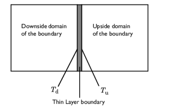
To evaluate the normal gradient operation, ∇n, temperatures Tu and Td are introduced for the upside and downside of the thin structure boundary. They are defined from the heat flux across the thin resistive structure. At the middle of the thickness, the temperature, T1 ⁄ 2, is approximated by (1 ⁄ 2)(Tu + Td). The term ∇n ⋅ (−dsk∇nT) is then given by:

Similarly, the time-dependent term can be expressed using Tu and Td by:

Equations for all supported types of medium are presented in the next sections, Thin Layer, Thin Film, Fracture, and Thin Rod.

This formulation is provided by the Thermally thick approximation option of the Thin Layer (Heat Transfer Interface) and Solid (Heat Transfer in Shells Interface) feature. Figure 4-5 shows how Thin Layer (Heat Transfer Interface) and Solid (Heat Transfer in Shells Interface) splits the temperature into Tu and Td on interior boundaries:

On exterior boundaries, it introduces a new degree of freedom represented by the variable TextFace. Depending on whether the heat domain is on the upside or the downside of the boundary, TextFace, is equal to Tu or Td and the same thing goes for the dependent variable T. An example is illustrated in the figure below:

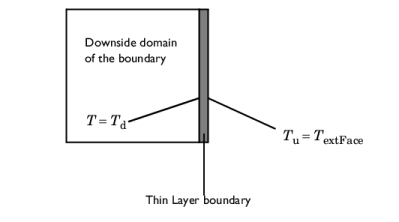
Table 4-3 summarizes the formulations available within the thin structure features of the Heat Transfer (ht) and Heat Transfer in Shells (htlsh) interfaces.