When the loading on a structure is random, and given by a PSD spectrum, a stress life approach can be used to assess fatigue using the Palmgren-Miner linear damage model (Ref. 3). The loading PSD will effectively produce a stress response PSD at every location in the structure, and this response PSD is used to assess fatigue. As the process is random, no finite time sample of the response will be identical to the next. Instead, assuming that any time sample is long enough, the statistics of each such sample should be the same, see
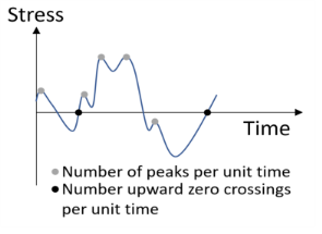
Random Vibration Theory for a detailed discussion. Statistical properties that are meaningful to a fatigue analysis include the number of upward zero crossings per unit time
n0, and the number of peaks per unit time
np.
Figure 3-27 shows a schematic of a stress time sample.
where G(
f) is the stress response PSD, and
f is the frequency. In particular, the zeroth moment
m0 is related to the RMS of the stress response through
The number of upward zero crossings per unit time n0, the number of peaks per unit time
np, and the irregularity factor
γ can be expressed in terms of the moments of the stress response spectrum as
In a fatigue analysis in the time domain, the Palmgren-Miner damage summation rule is often used in conjunction with a rainflow stress counting algorithm, with a discrete binning of stresses into a stress histogram, see the section on the Cumulative Damage Model for an overview. In the case of fatigue during random vibrations, the discrete stress histogram is replaced by a continuous, normalized probability density distribution function
P(
S), where
S is a stress amplitude. A requirement for
P(
S) is that if it is integrated from zero to infinity, for the total probability, the value is equal to one. The number of stress cycles
n(
S) at a given stress level
S is
where tp is the duration of the random vibration process. Note, that the probability of exactly an amplitude stress
S is zero, and in order to compute fatigue damage, we must use the Palmgren-Miner damage summation in a continuous sense, and integrate over all stress amplitudes:
Hence, the fatigue usage factor fus is computed by integrating the damage at each stress amplitude level, from zero to infinity. In practice, the infinite upper integration limit can be replaced by a sufficiently large, but finite value. The probability density distribution function diminishes at high stress levels, making it increasingly improbable to experience these stresses. In the expression above,
N(
S) is the expected number of cycles to failure at stress amplitude
S, as dictated by the specific fatigue model and the fatigue properties of the structural material in the structure. The function N(S) is defined by, for example, an S-N curve or the Basquin model. A fatigue usage factor exceeding one usually means that the structure fails due to fatigue.
The probability density distribution function P(
S) can be described using different models. These functions are essentially what define the counting of stress cycles, and depending on the characteristics of the stress response spectrum, a certain model may be more suitable than another. In this section, the models implemented in COMSOL Multiphysics are described.
In 1964, Bendat (Ref. 8) presented a theory for predicting fatigue damage due to random vibrations. This model is suitable for fatigue analyses of narrow band stress response spectra. In practice, this may a limitation in its applicability to more general spectra, as it tends to be overly conservative. The number of stress cycles
n(
S) at an amplitude stress level
S, using Bendat’s model, is given by
The model by Dirlik (Ref. 9) is empirical and it was developed based on Monte Carlo simulations. The Dirlik model is suitable for more general stress response spectra, and it is not limited to narrow band spectra, as is the Bendat model. The number of stress cycles
n(
S) at an amplitude stress level
S, using the Dirlik model, is given by
In practice, it is desirable to devise methods to account for the multiaxiality of the stress state. Preumont and Piéfort (Ref. 10) developed a method, in which a so-called
equivalent von Mises stress is used. This method has been implemented in COMSOL Multiphysics, and it is described below.
where σ is the stress vector with components, using standard notation,
σx,
σy,
σz,
σxy,
σyz, and
σxz, and the matrix
Q is given by
In this equation, E[
σσT] is the covariance matrix of the stress vector
σ. It is given by
where Gσσ(
f) is the PSD matrix of the stress vector. Next, a PSD
GEVMS(
f) is expressed based on the von Mises stress quadratic form such that
Note that this PSD is not the PSD of the von Mises stress itself, but by construction, it shares the mean square value. Thus,
Preumont and Piéfort define this to be a Gaussian random process such that
holds. By construction, the GEVMS(
f) PSD has a zero mean value, and it reduces to the correct, alternating stress in the case of pure uniaxial loading. The PSD function definition in
Equation 3-11is used to define the corresponding spectral moments of stress. The
k:th moment is defined as


