Periodic Boundary Conditions

To add a periodic boundary condition, in the , right-click a physics interface node and select . The periodic boundary condition typically implements standard periodicity so that u(x0) = u(x1) (that is, the value of the solution is the same on the periodic boundaries). In most cases you can also choose antiperiodicity so that the solutions have opposing signs: u(x0) = −u(x1). Other options such as Floquet periodicity or cyclic symmetry may be available. The periodicity is implemented in such a way that fluxes become periodic in the same way as the solution itself.

For fluid flow physics interfaces, the provides a similar periodic boundary condition but without a selection of periodicity. Instead, it allows specifying a pressure difference between the source and destination boundaries.

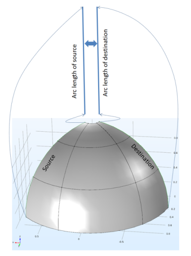
Typically, the periodic boundary conditions determine the source and destination boundaries automatically, but you can also add subnode to manually split the periodic boundary condition’s selection into source and destination selections.

	The KdV Equation and Solitons: Application Library path COMSOL_Multiphysics/Equation_Based/kdv_equation.

The periodic condition applies a constraint on the destination selection, constraining the solution at each destination point rdst to be equal to the solution at a corresponding source point rsrc. When the periodic condition is applied on surfaces in 3D or edges in 2D, the source point is computed using a rotation of the position relative to the destination and source centers of mass, r0,dst and r0,src:

where R is a rotation matrix encoding the relative orientation of the source and destination boundaries. It is normally determined automatically from the cross product of the source and destination boundary normal directions. That is, the rotation is performed about an axis perpendicular to the plane spanned by the normal directions, which are evaluated at arbitrary points on each boundary.

When the periodic condition is applied on a shell or beam in 3D, the selection is edges or vertices without a well-defined normal. An automatic mapping from destination point to source point is defined based on the geometry parameterization. Each destination point is mapped on a source point with the same arc length parameter value (see the image below).

The automatically computed relative orientation is in most cases the one expected. In particular, it is correct if the source and destination have unique normal vectors which are parallel but pointing in opposite directions, unless the geometry is twisted about that direction. But there are a number of situations when the automatic orientation is not necessarily the one expected:

For most periodic boundary conditions in the physics interfaces, it is then possible to specify the relative orientation of the source and destination selections using coordinate systems.

The orientation settings appear in an section in the main periodic condition node and in an section in a subnode. To display these settings, first select in the dialog box. The section is only visible if the source orientation has been chosen manually.

In both sections, there is a list. In the section in the main periodic condition node, its default value is . Other possible values represent coordinate systems, including all coordinate system nodes defined in the component as well as the canonical . The latter is the default choice for the section in subnodes.

The chosen source and destination coordinate systems define transformation matrices, Tsrc and Tdst, whose row index refers to local coordinate system components, while the column index refers to global coordinates on the source and destination selections, respectively. A rotation matrix as defined by Equation 3-2 is computed by assuming that the source and destination coordinate system coordinates refer to the same basis:

Some physics require that the meshes at that source and the destination are compatible. Here, compatible meshes means two meshes that can be mapped to each other (node points to node points) by an affine transformation. To make sure that source and destination are compatible you could, for instance, use the Copy mesh command. Sometimes the discretization requires even stronger assumptions than compatible meshes — the mapping needs to ensure that the mapped point is not only mapped to the correct physical point but also to the correct mesh element for the node points that are shared between adjacent mesh elements. The elementwise mapping for compatible meshes fulfills this requirement. One example that require the elementwise mapping is modeling of electromagnetic waves using curl type 2 shape functions (whereas for type 1 curl shape functions it is sufficient just to ensure that the meshes are indeed compatible).

In general, the constraint method is recommended for periodic conditions. When the constraint method is used for periodic conditions, the elementwise mapping for compatible meshes can lead to locking effects. This problem can be prevented by setting the value of the list to when the constraint method is used.

There is built-in logic for choosing if the software should try to use the elementwise mapping between the meshes or not. This corresponds to choosing from the list.

However, that logic is mainly based on the topology and does not consider the meshing sequence that you choose, the constraint method you set, or all the shape functions you will apply the condition to. Therefore, you can overwrite the built-in logic by choosing between the following alternatives from the list: , , or .

•

Choose if you expect compatible meshes and want to use an elementwise mapping but you want to get a mapping even if source and destination cannot be identified.

•

Choose if you do not expect compatible meshes or if you want to use elemental constraints for continuous fields.

•

Choose if you expect compatible meshes and you rather fail than use noncompatible meshes.