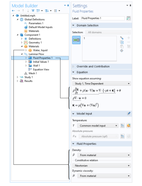
Figure 5 shows the Model Builder, including a Laminar Flow interface, and the Settings window for the selected Fluid Properties 1 feature node. The Fluid Properties 1 node adds the marked terms to the component equations in a selected geometry domain. Furthermore, the Fluid Properties 1 feature may link to the Materials feature node to obtain physical properties such as density and dynamic viscosity, in this case the fluid properties of water. The fluid properties, defined by the Water, liquid material, can be functions of the modeled physical quantities, such as pressure and temperature. In the same way, the Wall 1 node adds the boundary conditions at the walls of the fluid domain.

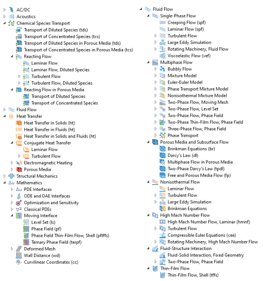
Figure 6 shows the Fluid Flow interfaces as they are displayed when you add a physics interface in 3D (see also Physics Interface Guide by Space Dimension and Study Type for further information). A short description of the physics interfaces follows.

The physics interfaces under the Turbulent Flow branch () model flows at high Reynolds numbers. These physics interfaces solve the Reynolds-averaged Navier–Stokes (RANS) equations for the averaged velocity and pressure fields. The turbulent flow interfaces provide different options for modeling the turbulent viscosity. There are several turbulence models available—two algebraic turbulence models, the Algebraic yPlus and L-VEL models, and seven transport-equation models, including a standard k-ε model, the Realizable k-ε model, a k-ω model, an SST (Shear Stress Transport) model, a low Reynolds number k-ε model, the Spalart–Allmaras model, and the v2-f model. Similarly to the Laminar Flow interface, incompressible flow is selected by default.

Among the transport-equation turbulence models, the standard k-ε model is the most widely used since it often is a good compromise between accuracy and computational cost (memory and CPU time). The Realizable k-ε model is similar to the standard k-ε model but has built-in realizability constraints, resulting in improved performance for certain flows, such as turbulent jets. The k-ω model is an alternative to the standard k-ε model and often gives more accurate results, especially in recirculation regions and close to solid walls. However, the k-ω model is also less robust than the standard k-ε model.

The SST model combines the robustness of the k-ε model with the accuracy of the k-ω model, making it applicable to a wide variety of turbulent flows. The Low Reynolds number k-ε model is more accurate than the standard k-ε model, especially close to walls.

In the v2-f model, the turbulent viscosity is based on the wall-normal velocity fluctuations, whereby wall blockage effects and low Reynolds number effects are captured separately. The v2-f model also includes non-local effects of the fluctuating pressure on the turbulent fields. Higher resolution is needed in the near-wall region for the SST model, the Low Reynolds number k-ε model, the Spalart-Allmaras model, and the v2-f model. Thus, the better accuracy provided by these models comes at a higher computational cost.

The Rotating Machinery interfaces () combine the Single-Phase Flow interfaces and a Rotating Domain, and are applicable to fluid-flow problems where one or more of the boundaries rotate, for example in mixers and around propellers. The physics interfaces support incompressible, weakly compressible and compressible (Mach < 0.3) flows, laminar Newtonian and non-Newtonian flows, and turbulent flow using the standard k-ε model or either of the two algebraic turbulence models (Algebraic yPlus or L-VEL).

The Euler-Euler Model interface () for two-phase flow is able to handle the same cases as the Bubbly Flow and Mixture Model interfaces, but is not limited to low concentrations of the dispersed phase. In addition, the Euler-Euler Model interface can handle large differences in density between the phases, such as the case of solid particles in air. This makes the model suitable for simulations of, for example, fluidized beds. There is support for both laminar flow and turbulent flow using either a mixture or phase-specific k-ε turbulence model.

The Nonisothermal Flow, Turbulent Flow interfaces () solve the Reynolds-Averaged Navier–Stokes (RANS) equations coupled to heat transfer in fluids and in solids. There is support for all the fluid-flow turbulence models – the Algebraic yPlus model, the L-VEL model, the standard k-ε model, the Realizable k-ε model, a k-ω model, an SST model, a low Reynolds number k-ε model, the Spalart-Allmaras model, and the v2-f model.

The High Mach Number Flow, Turbulent Flow interfaces () solve the continuity, momentum and energy equations for the averaged flow variables in fully compressible turbulent flow, coupled to transport equations for the turbulence quantities. There are two versions: one that uses to the k-ε turbulence model and one that uses to the Spalart-Allmaras turbulence model.

The Rotating Machinery, High Mach Number Flow interfaces () combine the High Mach Number Flow interfaces and a Rotating Domain, and are applicable to fluid-flow problems where one or more of the boundaries rotate, for example in turbines and around propellers. The physics interfaces support compressible, laminar, and turbulent flow using the k-ε model or the Spalart-Allmaras model.

The Turbulent Flow interfaces () and the Turbulent Flow, Diluted Species interfaces () under the Reacting Flow branch apply the Reynolds-Averaged Navier–Stokes (RANS) equations together with the functionality in the Transport of Concentrated Species interface or Transport of Diluted Species respectively. They model mass and momentum transport in turbulent reacting fluid flow. The supported RANS models include the standard k-ε model, a k-ω model, the SST model, and a low Reynolds number k-ε model.