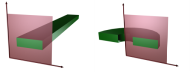
In this case you view a cross section in the xy-plane of the actual 3D geometry. The geometry is mathematically extended to infinity in both directions along the z-axis, assuming no variation along that axis. All the total flows in and out of boundaries are per unit length along the z-axis. A simplified way of looking at this is to assume that the geometry is extruded one unit length from the cross section along the z-axis. The total flow out of each boundary is then from the face created by the extruded boundary (a boundary in 2D is a line).

The spatial coordinates are called r and z, where r is the radius. The flow at the boundaries is given per unit length along the third dimension. Since this dimension is a revolution, you have to multiply all flows with αr, where α is the revolution angle (for example, 2π for a full turn).

Given that the necessary approximations are small, the solution is more accurate in 2D because a much denser mesh can be used. See 2D Problems if this is applicable.

You can use this approach either to convert 3D to 2D or to convert a layer to a boundary condition (see Simplifying the Geometry Using Boundary Conditions).