Newtonian and Non-Newtonian Fluids
A fluid may be characterized according to its response under the action of a shear stress. A Newtonian fluid has a linear relationship between shear stress and shear rate with the line passing through the origin. The constant of proportionality is referred to as the viscosity of the fluid and may depend on temperature, pressure and composition. For a non-Newtonian fluid, the curve for shear stress versus shear rate is nonlinear or does not pass through the origin. If the curve is shifted away from the origin, the fluid has a yield stress. If the curve bends towards the shear-rate axis, the fluid is said to be shear thinning (pseudoplastic), but if it instead bends towards the shear-stress axis, it is said to be shear thickening (dilatant). The relationship may also contain time derivatives of the shear rate to model memory effects (thixotropy), and even parallel viscous and elastic responses. We refer to the latter as viscoelastic non-Newtonian fluids and all others as inelastic non-Newtonian fluids. For the inelastic non-Newtonian models, it is possible to define an apparent viscosity from a generalized Newtonian relationship between the deviatoric stress tensor and the strain-rate tensor.
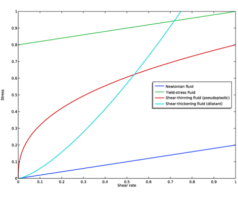
Figure 2-1:
Conceptual behavior of shear stress versus shear rate for Newtonian, yield-stress, shear-thinning and shear-thickening fluids.
The apparent viscosity will then be a function of the first invariant of the strain-rate tensor. In simple shear flows, this invariant simplifies to the shear rate.
The inelastic non-Newtonian models in the Polymer Flow Module are listed below:
•
Bingham–Papanastasiou (Viscoplastic)
•
Casson–Papanastasiou (Viscoplastic)
•
Power Law
•
Carreau
•
Carreau–Yasuda
•
Cross
•
Cross-Williamson
•
Ellis
•
Herschel–Bulkley–Papanastasiou
•
Robertson–Stiff–Papanastasiou
•
DeKee–Turcotte–Papanastasiou
•
Houska thixotropy (Thixotropic)
The Bingham-Papanastasiou and Casson–Papanastasiou models are yield-stress fluids with a linear behavior at high shear rates. The Power Law model can be used to study both shear-thinning and shear-thickening behavior. The Carreau, Carreau-Yasuda and Cross models are appropriate for shear-thinning fluids when there is a significant deviation from the Power Law model at very high and very low shear rates. Similarly, the Cross-Williamson and Ellis models can be used to study shear-thinning behavior when the deviations from the Power Law model are significant only at low shear rates. Herschel–Bulkley–Papanastasiou and Robertson–Stiff–Papanastasiou are power-law fluids with a yield-stress. The DeKee–Turcotte–Papanastasiou model is a yield-stress fluid with an exponential shear-thinning behavior at high shear rates. For the Houska thixotropy model, the apparent viscosity decreases with the time of shearing. Its structure breaks down under shear and rebuilds at rest. Thixotropic fluids display a hysteresis loop in the shear-rate shear-stress plane. The Houska model also includes a yield stress.
The viscoelastic models in the Polymer Flow Module are:
•
Oldroyd-B
•
Giesekus
•
FENE-P
•
LPTT
The simplest one is the Oldroyd-B model which has a constant viscosity and a constant first normal-stress coefficient. This is conceptually visualized as a Hookean spring in series with a dash-pot in
To ensure material-frame indifference, an upper-convected time derivative is used to describe the transport of the additional stress due to the spring and dash-pot. Multiple branches with different relaxation times and viscosities can be added in order to include multi-modal responses. In the Oldroyd-B model, the springs are infinitely extensible, which can lead to unphysical behavior. The Giesekus model adds a quadratic stress term, thereby capturing power-law behavior in the viscous and normal stress components. The FENE-P (Finitely Extensible Nonlinear Elastic with the Peterlin approximation) model includes nonlinear-spring behavior and shear thinning. Extension hardening and shear thinning can be studied with the LPTT (Linear Phan-Thien/Tanner) model.
When applying a viscoelastic model, it is important to keep in mind that the mathematical formulation may become ill posed at sharp corners. One remedy is to use a fillet operation to smooth the geometry at such points. As always when working with complex fluid flow simulations, it is advisable to start with a simple model, and then switch to a more complicated model if the simple model does not capture the expected flow phenomena. In most industrial applications, inelastic non-Newtonian models produce sufficiently accurate results at a reasonable computational cost.