You are viewing the documentation for an older COMSOL version. The latest version is
available here
.
The Polymer Flow Module
Non-Newtonian fluids are found in a great variety of processes in the polymer, food, pharmaceutical, cosmetics, household, and fine chemicals industries. Examples of these fluids are coatings, paints, yogurt, ketchup, colloidal suspensions, aqueous suspensions of drugs, lotions, creams, shampoo, suspensions of peptides and proteins, to mention a few. The Polymer Flow Module is an optional add-on package for COMSOL Multiphysics designed to aid engineers and scientists in simulating flows of non-Newtonian fluids with viscoelastic, thixotropic, shear thickening, or shear thinning properties. Simulations can be used to gain physical insight into the behavior of complex fluids, reduce prototyping costs, and to speed up development. The Polymer Flow Module allows users to quickly and accurately model single-phase flows, multiphase flows, nonisothermal flows, and reacting flows of Newtonian and non-Newtonian fluids.
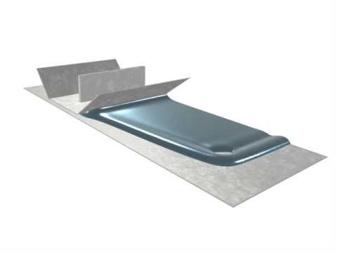
Figure 1:
Coating flow simulation with a power-law fluid. The thickness of the coating layer can be controlled by varying the speed of the lower wall relative to that of the injection slot. Span-wise thickness variations and edge effects may be minimized by optimizing the polymer composition in the coating fluid.
The Polymer Flow Module can solve stationary and time-dependent flows in two-dimensional and three-dimensional domains. Formulations suitable for different types of flow are set up as predefined Fluid Flow interfaces, referred to as physics interfaces. These Fluid Flow interfaces use physical quantities, such as velocity and pressure, and physical properties, such as density and viscosity, to define a fluid-flow problem. Different physics interfaces are available to cover a range of flows. Examples include: Laminar Flow, Creeping Flow, Viscoelastic Flow, Heat Transfer, and Transport of Diluted Species. The physics interfaces can be combined with the interfaces in the Mathematics branch (Level Set, Phase Field and Ternary Phase Field), or defined on an Arbitrary Lagrangian Eulerian (ALE) frame to simulate two- and three-phase flows, and rotating flows. The Polymer Flow Module includes a set of predefined multiphysics couplings, including: Nonisothermal Flow; Reacting Flow; Two-Phase Flow, Level Set; Two-Phase Flow, Phase Field; Three-Phase Flow, Phase Field; and Rotating Machinery, Fluid Flow, to facilitate the setup of multiphysics simulations.
For each of the physics interfaces, the underlying physical principles are expressed in the form of partial differential equations, together with corresponding initial and boundary conditions. COMSOL’s design emphasizes the physics by providing users with the equations solved by each feature and offering the user full access to the underlying equation system. There is also tremendous flexibility to add user-defined equations and expressions to the system. For example, to model the curing state during a mold injection, a Stabilized Convection Diffusion Equation interface can be added from the Mathematics branch—no scripting or coding is required. When COMSOL compiles the equations the complex couplings generated by these user-defined expressions are automatically included in the equation system. The equations are then solved using the finite element method and a range of industrial-strength solvers. Once a solution is obtained a vast range of postprocessing tools are available to analyze the data, and predefined plots are automatically generated to visualize the results. COMSOL offers the flexibility to evaluate a wide range of physical quantities including predefined quantities such as the pressure, velocity, shear rate, or the vorticity (available through easy-to-use menus), as well as arbitrary user-defined expressions.
To set up a fluid flow simulation, the geometry is first defined in the software. Then appropriate materials are selected and suitable physics interfaces together with the appropriate multiphysics couplings are added. Initial conditions and boundary conditions are set up within the physics interfaces. Next, the mesh is defined—in many cases COMSOL’s default mesh, which is produced from physics-dependent defaults, will be appropriate for the problem. A solver is selected, again with defaults appropriate for the relevant physics interfaces, and the problem is solved. Finally the results are visualized. All these steps are accessed from the COMSOL Desktop.