PDF

Time to Frequency FFT Analysis of a Distributed Bragg Reflector
Introduction
A distributed Bragg reflector (DBR), or dielectric mirror, is a structure used in bulk optics and waveguides to reflect light. It has extremely low losses at optical and infrared frequencies compared to ordinary metallic mirrors. The structure is formed from alternating thin layers of materials with high and low refractive indices, where each layer is one quarter of a material wavelength thick.
Figure 1: The distributed Bragg reflector structure. The first layer represents the infinite superstrate. In this case air is used. The high-index layers are made of titanium dioxide and the low-index layers use silica. Also the substrate is assumed to use silica.
Each layer boundary causes a partial reflection of an optical wave. When the wavelength is close to four times the optical thickness of the layers, the many reflected waves tend to interfere constructively, causing the layers to act as a high-quality reflector. The range of wavelengths in which most of the incident intensity is reflected is called the photonic stopband. In the limit in which the reflector contains a very large number of layers, radiation in this range of wavelengths cannot propagate into the structure.
Distributed Bragg reflectors are critical components in for instance vertical cavity surface emitting lasers (see Threshold Gain Calculations for Vertical-Cavity Surface-Emitting Lasers (VCSELs)).
This model demonstrates how to setup a Time to Frequency FFT study for a distributed Bragg reflector (DBR) structure. It also compares the results with results from a regular Frequency domain study.
Model Definition
The model consists of a structure of twenty periods of alternating high and low refractive index layers. The refractive indexes are tabulated in Table 1 below.
Each layer is a quarter of a material wavelength thick.
In the first study, a modulated Gaussian pulse is used for exciting the structure. The input electric field for the Scattering boundary condition is defined by
,
where E0 is the amplitude, t is time, Td = 1/(2f0) is the pulse duration, f0 is the center frequency, Tc = 3Td is a delay time, ω0 = 2πf0 is the center angular frequency, and z is the unit vector in the z-direction.
In a Time to Frequency FFT, the time dependent solution, from an initial Time Dependent study step, is transformed to a frequency dependent solution. To make it possible to also perform an FFT on the input electric field above, a dependent variable is assigned the value of the input electric field function. Then the FFT is performed also on that dependent variable.
To generate the frequency-domain data without significant distortion in the frequency range between 0 and 2f0, the time step, satisfying the Nyquist criterion, is set to 1/4f0 = 1/2B, where B is the bandwidth 2f0.
Results and Discussion
Figure 1 shows the electric field distribution in the DBR structure. The plot is calculated using an FFT of the time dependent solution. At the center frequency for the stop band, the field decays quickly in the structure. Almost no field is transmitted.
Figure 2: The electric field distribution at the center of the stopband (300 THz). The plot is calculated by performing an FFT of the time dependent solution.
As a comparison, Figure 3 shows a similar plot as in Figure 2, but calculated by a regular Frequency domain study. The two field distributions look the same, except for the different amplitudes.
Figure 3: The electric field distribution at the center of the stopband (299.9 THz), as computed by a Frequency domain study.
Figure 4 shows that the transmittance spectra for the two types of simulations agree very well.
Figure 4: The transmittance for the two type of simulations. The blue curve is performed by performing an FFT on the time domain solution, and the green curve is the result of a regular frequency sweep.
Figure 5 shows the field distribution after 40 fs. At that point in time, the main pulse has almost passed the mirror structure. As shown in Figure 6, the electromagnetic energy decays slowly, as the radiation is being reflected back and forth in the layer structure before it escapes through the left and right boundaries. However, at the end of the simulation, there is not much energy left in the structure. Thus, as shown in Figure 4, the result from the FFT of the time dependent signal is very accurate, as almost the whole time dependent phenomena is included in the simulation.
Figure 5: The electric field distribution after 40 fs, when the main pulse has almost propagated through the whole mirror structure.
Figure 6: The electromagnetic energy in the mirror structure versus time.
Application Library path: Wave_Optics_Module/Optical_Scattering/time_to_frequency_fft_distributed_bragg_reflector
Modeling Instructions
From the File menu, choose New.
New
In the New window, click  Model Wizard.
Model Wizard
1
In the Model Wizard window, click  2D.
2
In the Select Physics tree, select Optics>Wave Optics>Electromagnetic Waves, Transient (ewt).
3
Click Add.
4
In the Select Physics tree, select Optics>Wave Optics>Electromagnetic Waves, Frequency Domain (ewfd).
5
Click Add.
6
Click  Study.
7
In the Select Study tree, select Preset Studies for Selected Physics Interfaces>Electromagnetic Waves, Transient>Time Dependent with FFT.
8
Global Definitions
Parameters 1
Add some parameters that are used for configuring the geometry, the materials, the mesh, and the solvers.
1
In the Model Builder window, under Global Definitions click Parameters 1.
2
In the Settings window for Parameters, locate the Parameters section.
3
Click  Load from File.
4
Browse to the model’s Application Libraries folder and double-click the file time_to_frequency_fft_distributed_bragg_reflector_parameters.txt.
Geometry 1
Now, add the geometry. Define cumulative selections to make it easier to add the materials to the right layers.
Superstrate
1
In the Geometry toolbar, click  Rectangle.
2
In the Settings window for Rectangle, type Superstrate in the Label text field.
3
Locate the Size and Shape section. In the Width text field, type d0.
4
In the Height text field, type lda0.
5
Locate the Position section. In the x text field, type -d0.
High-Index Layer
1
Right-click Superstrate and choose Duplicate.
2
In the Settings window for Rectangle, type High-Index Layer in the Label text field.
3
Locate the Size and Shape section. In the Width text field, type dH.
4
Locate the Position section. In the x text field, type 0.
5
Locate the Selections of Resulting Entities section. Find the Cumulative selection subsection. Click New.
6
In the New Cumulative Selection dialog box, type High-Index Material in the Name text field.
7
Low-Index Layer
1
Right-click High-Index Layer and choose Duplicate.
2
In the Settings window for Rectangle, type Low-Index Layer in the Label text field.
3
Locate the Size and Shape section. In the Width text field, type dL.
4
Locate the Position section. In the x text field, type dH.
5
Locate the Selections of Resulting Entities section. Find the Cumulative selection subsection. Click New.
6
In the New Cumulative Selection dialog box, type Low-Index Material in the Name text field.
7
Period
1
In the Geometry toolbar, click  Booleans and Partitions and choose Union.
2
In the Settings window for Union, type Period in the Label text field.
3
Select the objects r2 and r3 only.
Array 1 (arr1)
1
In the Geometry toolbar, click  Transforms and choose Array.
2
3
In the Settings window for Array, locate the Size section.
4
In the x size text field, type NPeriod.
5
Locate the Displacement section. In the x text field, type dPeriod.
Final High-Index Layer
1
In the Model Builder window, under Component 1 (comp1)>Geometry 1 right-click High-Index Layer (r2) and choose Duplicate.
2
In the Settings window for Rectangle, type Final High-Index Layer in the Label text field.
3
Locate the Position section. In the x text field, type L_tot-dH.
Substrate
1
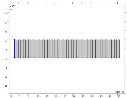
In the Model Builder window, under Component 1 (comp1)>Geometry 1 right-click Superstrate (r1) and choose Duplicate.
2
In the Settings window for Rectangle, type Substrate in the Label text field.
3
Locate the Size and Shape section. In the Width text field, type ds.
4
Locate the Position section. In the x text field, type L_tot.
5
Locate the Selections of Resulting Entities section. Find the Cumulative selection subsection. From the Contribute to list, choose Low-Index Material.
6
Click  Build All Objects.
7
Click the  Zoom Extents button in the Graphics toolbar.
Materials
Add the materials now, using the cumulative selections defined with the geometry.
Air
1
In the Model Builder window, under Component 1 (comp1) right-click Materials and choose Blank Material.
2
In the Settings window for Material, type Air in the Label text field.
3
Locate the Material Contents section. In the table, enter the following settings:
By default, the first added material will have All domains as the selection. The materials added later will override all selected domains, except for the leftmost superstrate domain.
Titanium Dioxide
1
Right-click Materials and choose Blank Material.
2
In the Settings window for Material, type Titanium Dioxide in the Label text field. This will be the high-index material.
3
Locate the Geometric Entity Selection section. From the Selection list, choose High-Index Material.
4
Locate the Material Contents section. In the table, enter the following settings:
Silica
1
Right-click Materials and choose Blank Material.
2
In the Settings window for Material, type Silica in the Label text field. This will be the low-index material.
3
Locate the Geometric Entity Selection section. From the Selection list, choose Low-Index Material.
4
Locate the Material Contents section. In the table, enter the following settings:
Definitions
Next, add the modulated Gaussian input electric field.
Modulated Gaussian Input Field
1
In the Home toolbar, click  Functions and choose Local>Analytic.
2
In the Settings window for Analytic, type Modulated Gaussian Input Field in the Label text field.
3
In the Function name text field, type Ein.
4
Locate the Definition section. In the Expression text field, type E0*exp(-(t-Tc)^2/Td^2)*sin(omega0*(t-Tc)).
5
In the Arguments text field, type t.
6
Locate the Units section. In the Arguments text field, type s.
7
In the Function text field, type V/m.
Top Exterior Boundaries
Before adding the physics, it is useful to add some selections that will be used by the physics features.
1
In the Definitions toolbar, click  Explicit.
2
In the Settings window for Explicit, type Top Exterior Boundaries in the Label text field.
3
Locate the Input Entities section. From the Geometric entity level list, choose Boundary.
4
Click the  Select Box button in the Graphics toolbar.
5
Bottom Exterior Boundaries
1
Right-click Top Exterior Boundaries and choose Duplicate.
2
In the Settings window for Explicit, type Bottom Exterior Boundaries in the Label text field.
3
Locate the Input Entities section. Click  Clear Selection.
4
Click the  Select Box button in the Graphics toolbar.
5
Top and Bottom Exterior Boundaries
1
In the Definitions toolbar, click  Union.
2
In the Settings window for Union, type Top and Bottom Exterior Boundaries in the Label text field.
3
Locate the Geometric Entity Level section. From the Level list, choose Boundary.
4
Locate the Input Entities section. Under Selections to add, click  Add.
5
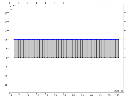
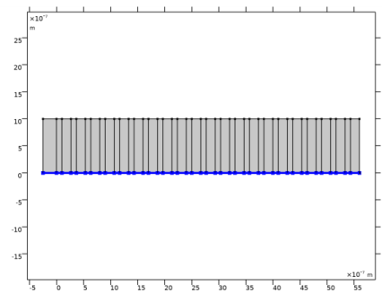
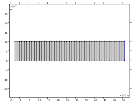
In the Add dialog box, in the Selections to add list, choose Top Exterior Boundaries and Bottom Exterior Boundaries.
6
Top High-Index Material Boundaries
1
In the Definitions toolbar, click  Intersection.
2
In the Settings window for Intersection, type Top High-Index Material Boundaries in the Label text field.
3
Locate the Geometric Entity Level section. From the Level list, choose Boundary.
4
Locate the Input Entities section. Under Selections to intersect, click  Add.
5
In the Add dialog box, in the Selections to intersect list, choose Top Exterior Boundaries and High-Index Material.
6
Top Low-Index Material Boundaries
1
Right-click Top High-Index Material Boundaries and choose Duplicate.
2
In the Settings window for Intersection, type Top Low-Index Material Boundaries in the Label text field.
3
Locate the Input Entities section. In the Selections to intersect list, select High-Index Material.
4
Under Selections to intersect, click  Delete.
5
Under Selections to intersect, click  Add.
6
In the Add dialog box, select Low-Index Material in the Selections to intersect list.
7
Domain Point Probe 1
A probe will be added to visualize the progress while solving.
1
In the Definitions toolbar, click  Probes and choose Domain Point Probe.
2
In the Settings window for Domain Point Probe, locate the Point Selection section.
3
In row Coordinates, set x to L_tot+ds, to select the point in the lower right corner.
4
Select the Snap to closest boundary check box.
Point Probe Expression 1 (ppb1)
1
In the Model Builder window, expand the Domain Point Probe 1 node, then click Point Probe Expression 1 (ppb1).
2
In the Settings window for Point Probe Expression, locate the Expression section.
3
In the Expression text field, type ewt.Ez.
Integration 1 (intop1)
Add a few integration operators that will be used for calculating the input and transmitted powers, and the energy stored in the mirror structure.
1
In the Definitions toolbar, click  Nonlocal Couplings and choose Integration.
2
In the Settings window for Integration, locate the Source Selection section.
3
From the Geometric entity level list, choose Boundary.
4
Integration 2 (intop2)
1
Right-click Integration 1 (intop1) and choose Duplicate.
2
In the Settings window for Integration, locate the Source Selection section.
3
Click  Clear Selection.
4
Integration 3 (intop3)
1
In the Definitions toolbar, click  Nonlocal Couplings and choose Integration.
2
In the Settings window for Integration, locate the Source Selection section.
3
From the Selection list, choose All domains.
Variables 1
Add variables for the input power and the transmitted power, using the integration operators defined above.
1
In the Model Builder window, right-click Definitions and choose Variables.
2
In the Settings window for Variables, locate the Variables section.
3
Electromagnetic Waves, Transient (ewt)
1
In the Model Builder window, under Component 1 (comp1) click Electromagnetic Waves, Transient (ewt).
2
In the Settings window for Electromagnetic Waves, Transient, locate the Components section.
3
From the Electric field components solved for list, choose Out-of-plane vector, to solve for only the out-of-plane (z) polarization.
Scattering Boundary Condition 1
1
In the Physics toolbar, click  Boundaries and choose Scattering Boundary Condition.
2
3
In the Settings window for Scattering Boundary Condition, locate the Scattering Boundary Condition section.
4
From the Incident field list, choose Wave given by E field.
5
Specify the E0 vector as
Scattering Boundary Condition 2
1
In the Physics toolbar, click  Boundaries and choose Scattering Boundary Condition.
2
Perfect Magnetic Conductor 1
1
In the Physics toolbar, click  Boundaries and choose Perfect Magnetic Conductor.
2
In the Settings window for Perfect Magnetic Conductor, locate the Boundary Selection section.
3
From the Selection list, choose Top and Bottom Exterior Boundaries.
Add a dependent variable representing the input electric field. This will make it possible to perform an FFT on that variable. However, to be able to add the dependent variable, using a Global Equation node, the Equation-Based Contributions checkbox must be enabled in the Show More Options dialog.
4
Click the  Show More Options button in the Model Builder toolbar.
5
In the Show More Options dialog box, in the tree, select the check box for the node Physics>Equation-Based Contributions.
6
Global Equations 1
1
In the Physics toolbar, click  Global and choose Global Equations.
2
In the Settings window for Global Equations, locate the Global Equations section.
3
This will make the dependent variable EinODE follow the input electric field, defined by the function Ein(t).
4
Locate the Units section. Click  Select Dependent Variable Quantity.
5
In the Physical Quantity dialog box, type electric in the text field.
6
Click  Filter.
7
In the tree, select Electromagnetics>Electric field (V/m).
8
9
In the Settings window for Global Equations, locate the Units section.
10
Click  Select Source Term Quantity.
11
In the Physical Quantity dialog box, click OK, to select the Electric field.
Mesh 1
Now, add a very fine mesh that resolves also the higher frequencies properly.
Size 1
1
In the Model Builder window, under Component 1 (comp1) right-click Mesh 1 and choose Size.
2
In the Settings window for Size, locate the Geometric Entity Selection section.
3
From the Geometric entity level list, choose Boundary.
4
5
Locate the Element Size section. Click the Custom button.
6
Locate the Element Size Parameters section. Select the Maximum element size check box.
7
Size 2
1
Right-click Size 1 and choose Duplicate.
2
In the Settings window for Size, locate the Geometric Entity Selection section.
3
From the Selection list, choose Top High-Index Material Boundaries.
4
Locate the Element Size Parameters section. In the Maximum element size text field, type lda0/2/nH/20.
Size 3
1
Right-click Size 2 and choose Duplicate.
2
In the Settings window for Size, locate the Geometric Entity Selection section.
3
From the Selection list, choose Top Low-Index Material Boundaries.
4
Locate the Element Size Parameters section. In the Maximum element size text field, type lda0/2/nL/20.
Edge 1
1
In the Mesh toolbar, click  Edge.
2
In the Settings window for Edge, locate the Boundary Selection section.
3
From the Selection list, choose Top Exterior Boundaries.
Copy Edge 1
1
In the Model Builder window, right-click Mesh 1 and choose More Operations>Copy Edge.
2
In the Settings window for Copy Edge, locate the Source Boundaries section.
3
From the Selection list, choose Top Exterior Boundaries.
4
Locate the Destination Boundaries section. From the Selection list, choose Bottom Exterior Boundaries.
Distribution 1
1
Right-click Mesh 1 and choose Distribution.
2
3
In the Settings window for Distribution, locate the Distribution section.
4
In the Number of elements text field, type 1.
Mapped 1
1
In the Mesh toolbar, click  Mapped.
2
In the Settings window for Mapped, click  Build All.
Study 1
Step 1: Time Dependent
1
In the Model Builder window, under Study 1 click Step 1: Time Dependent.
2
In the Settings window for Time Dependent, locate the Study Settings section.
3
From the Time unit list, choose fs.
4
In the Output times text field, type range(0,0.25*T0,Tmax).
5
Locate the Physics and Variables Selection section. In the table, clear the Solve for check box for Electromagnetic Waves, Frequency Domain (ewfd).
Step 2: Time to Frequency FFT
1
In the Model Builder window, click Step 2: Time to Frequency FFT.
2
In the Settings window for Time to Frequency FFT, locate the Study Settings section.
3
From the Time unit list, choose fs.
4
In the End time text field, type Tend.
5
From the Frequency unit list, choose THz.
6
In the Maximum output frequency text field, type 2*f0.
7
Locate the Physics and Variables Selection section. In the table, clear the Solve for check box for Electromagnetic Waves, Frequency Domain (ewfd).
Step 3: Combine Solutions
1
In the Model Builder window, click Step 3: Combine Solutions.
2
In the Settings window for Combine Solutions, locate the Combine Solutions Settings section.
3
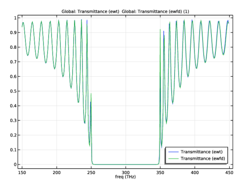
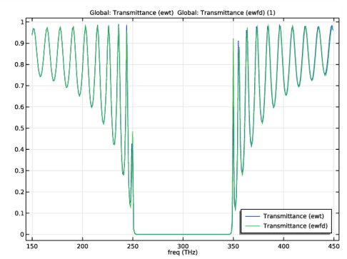
In the Excluded if text field, type freq<0.5*f0||freq>1.5*f0, to remove too low and too high frequencies.
Solution 1 (sol1)
Create the default solver sequence and then edit the time stepping to use a constant step size.
1
In the Study toolbar, click  Show Default Solver.
2
In the Model Builder window, expand the Solution 1 (sol1) node, then click Time-Dependent Solver 1.
3
In the Settings window for Time-Dependent Solver, click to expand the Time Stepping section.
4
From the Steps taken by solver list, choose Manual.
5
In the Time step text field, type 0.01*T0.
6
In the Study toolbar, click  Compute.
Results
Electric Field (ewt, FD)
1
In the Settings window for 2D Plot Group, type Electric Field (ewt, FD) in the Label text field.
2
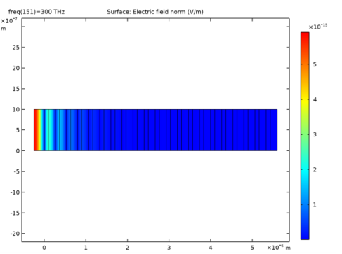
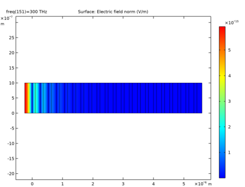
Locate the Data section. From the Parameter value (freq (THz)) list, choose 300, which is the center frequency (in the middle of the stopband).
3
In the Electric Field (ewt, FD) toolbar, click  Plot.
Electric Field (ewt, TD)
Add an additional plot group to visualize the time dependent solution.
1
In the Home toolbar, click  Add Plot Group and choose 2D Plot Group.
2
In the Settings window for 2D Plot Group, type Electric Field (ewt, TD) in the Label text field.
3
Locate the Data section. From the Dataset list, choose Study 1/Solution Store 1 (sol2).
Surface 1
1
Right-click Electric Field (ewt, TD) and choose Surface.
2
In the Settings window for Surface, locate the Expression section.
3
In the Expression text field, type ewt.Ez.
Electric Field (ewt, TD)
1
In the Model Builder window, click Electric Field (ewt, TD).
2
In the Settings window for 2D Plot Group, locate the Data section.
3
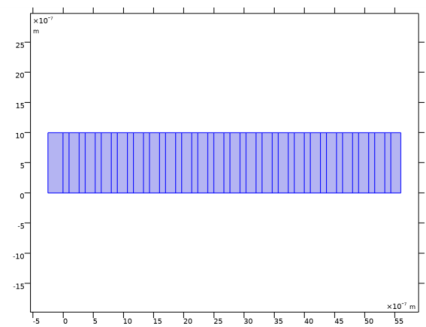
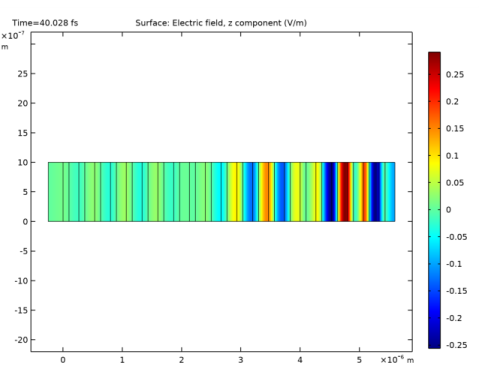
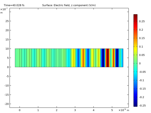
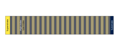
From the Time (fs) list, choose 40.028, showing the field distribution as the pulse has almost propagated through the mirror structure.
4
In the Electric Field (ewt, TD) toolbar, click  Plot.
Animation 1
In the Electric Field (ewt, TD) toolbar, click  Animation and choose Player, to display an animation of the temporal behavior of the field.
Transmittance
Add a plot group for displaying the transmittance versus frequency.
1
In the Home toolbar, click  Add Plot Group and choose 1D Plot Group.
2
In the Settings window for 1D Plot Group, type Transmittance in the Label text field.
Global 1
1
Right-click Transmittance and choose Global.
2
In the Settings window for Global, locate the y-Axis Data section.
3
Transmittance
1
In the Model Builder window, click Transmittance.
2
In the Settings window for 1D Plot Group, locate the Legend section.
3
From the Position list, choose Lower right.
4
In the Transmittance toolbar, click  Plot.
Energy
Verify that the energy has decayed from the mirror by the end of the simulation, by plotting the electromagnetic energy versus time.
1
In the Home toolbar, click  Add Plot Group and choose 1D Plot Group.
2
In the Settings window for 1D Plot Group, type Energy in the Label text field.
3
Locate the Data section. From the Dataset list, choose Study 1/Solution Store 1 (sol2).
4
Locate the Legend section. Clear the Show legends check box.
Global 1
1
Right-click Energy and choose Global.
2
In the Settings window for Global, locate the y-Axis Data section.
3
Energy
1
In the Model Builder window, click Energy.
2
In the Settings window for 1D Plot Group, locate the Axis section.
3
Select the y-axis log scale check box.
4
Select the Manual axis limits check box.
5
In the y minimum text field, type 1e-30.
6
In the Energy toolbar, click  Plot.
Indeed, there is almost no energy left in the mirror at the end of the simulation.
Electromagnetic Waves, Frequency Domain (ewfd)
Now, make a frequency domain simulation, to compare with the results from the time-to-frequency FFT analysis.
1
In the Model Builder window, under Component 1 (comp1) click Electromagnetic Waves, Frequency Domain (ewfd).
2
In the Settings window for Electromagnetic Waves, Frequency Domain, locate the Components section.
3
From the Electric field components solved for list, choose Out-of-plane vector.
Scattering Boundary Condition 1
1
In the Physics toolbar, click  Boundaries and choose Scattering Boundary Condition.
2
3
In the Settings window for Scattering Boundary Condition, locate the Scattering Boundary Condition section.
4
From the Incident field list, choose Wave given by E field.
5
Specify the E0 vector as
Scattering Boundary Condition 2
1
In the Physics toolbar, click  Boundaries and choose Scattering Boundary Condition.
2
Perfect Magnetic Conductor 1
1
In the Physics toolbar, click  Boundaries and choose Perfect Magnetic Conductor.
2
In the Settings window for Perfect Magnetic Conductor, locate the Boundary Selection section.
3
From the Selection list, choose Top and Bottom Exterior Boundaries.
Add Study
1
In the Home toolbar, click  Add Study to open the Add Study window.
2
Go to the Add Study window.
3
Find the Physics interfaces in study subsection. In the table, clear the Solve check box for Electromagnetic Waves, Transient (ewt).
4
Find the Studies subsection. In the Select Study tree, select General Studies>Frequency Domain.
5
Click Add Study in the window toolbar.
6
In the Home toolbar, click  Add Study to close the Add Study window.
Study 2
Step 1: Frequency Domain
1
In the Settings window for Frequency Domain, locate the Study Settings section.
2
In the Frequencies text field, type range(0.5*f0,deltaf,1.5*f0).
3
Click to expand the Results While Solving section. From the Probes list, choose None.
4
Locate the Physics and Variables Selection section. Select the Modify model configuration for study step check box.
5
In the Physics and variables selection tree, select Component 1 (comp1)>Electromagnetic Waves, Transient (ewt).
6
Click  Disable in Model.
7
In the Home toolbar, click  Compute.
Results
Electric Field (ewfd)
1
In the Settings window for 2D Plot Group, locate the Data section.
2
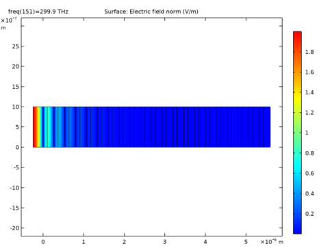
From the Parameter value (freq (THz)) list, choose 299.9, which is the center frequency in the sweep.
3
In the Electric Field (ewfd) toolbar, click  Plot.
Notice that the field distribution is the same as for the time-to-frequency FFT result, except that the amplitude is different.
Global 2
1
In the Model Builder window, right-click Transmittance and choose Global.
2
In the Settings window for Global, locate the Data section.
3
From the Dataset list, choose Probe Solution 4 (sol4).
4
Locate the y-Axis Data section. In the table, enter the following settings:
5
In the Transmittance toolbar, click  Plot.
The curves from the two studies agree very well.