Focusing Lens

It is challenging to simulate systems with optical lenses by the standard full vector wave analysis method because the number of mesh elements tends to be extremely large for the size of regular optical lenses. Since the standard frequency domain analysis solves for the electric field, the mesh needs to resolve the fast-oscillating field amplitude in order to get an accurate solution, that is, the maximum element size needs to be 1/5 of the wavelength or smaller. This standard method is suited for systems that are comparable to or up to ten times the wavelength. Compared to the standard method, the beam envelopes method is another type of full vector wave analysis that solves for the slowly varying envelope. With this method, the requirement for meshing is largely reduced depending on how slowly the envelope varies and therefore it is possible to solve systems with a large domain size. Lenses that are relatively smaller in size and are slow (focal length is not too small) may potentially be good candidates for the Electromagnetic Waves, Beam Envelopes interface in the Wave Optics Module, if the intensity computation is of interest.

In this model, a plano-convex focusing lens is analyzed by using the Electromagnetic Waves, Frequency Domain interface and the Electromagnetic Waves, Beam Envelopes interface. The computational results are compared. The Electromagnetic Waves, Frequency Domain interface analyzes only the lens domain and its vicinity. A boundary field at the exit plane of the lens is propagated to the focal plane by the Fresnel diffraction formula. The Electromagnetic Waves, Beam Envelopes interface analyzes the entire domain including the focal plane.

Model Definition

The plano-convex lens has a diameter of 0.2 mm, thickness of 15 μm, the radius of curvature of 0.5 mm, and the focal length of about 1 mm. The front surface of the lens is illuminated by a top-hat beam with a size of 0.1 mm, as depicted in Figure 1. This is a slow lens with a numerical aperture of about 0.05.

Figure 1: The optical layout.

The first study uses the Electromagnetic Waves, Frequency Domain interface to analyze the near field; that is, only the lens domain and its vicinity. After computing the near field, the electric field amplitude at the exit side of the lens is transformed to the focal plane by using the Fresnel diffraction formula (Ref. 1):

where λ is the wavelength; f is the focal length; and u/(λf) is called the spatial frequency; and E(x0, y) and E(f, u) are the electric field amplitudes at the exit plane x = x0 and at the focal plane x = f, respectively.

To evaluate the integral above, an integration operator intop1 is defined on the boundary at the exit plane. The y coordinate in the focal plane, the coordinate u, is defined by a one-dimensional grid dataset. To make sure that u is evaluated on the grid data set, and not on the exit plane boundary, the dest operator is applied to u. The dest operator forces the expression that it operates on to be evaluated on the destination points (the grid data set points in this case) instead of the source points (the exit plane boundary). This means that the destination operator (dest) can be used to create convolution integrals and other integral transforms.

The second study uses the Electromagnetic Waves, Beam Envelopes interface to solve for the electric field norm in the entire domain, including the focal plane. In this simulation, it should be emphasized that the mesh element is as large as λ in the air domain, compared to the first study, in which the Electromagnetic Waves, Frequency Domain interface requires a mesh element of λ/n/5 everywhere in the near-field domain.

For both physics interfaces, a Transition boundary condition is used for approximating an anti-reflection (AR) coating applied to the lens surfaces. The Transition boundary condition has the advantage that the thin AR coating doesn’t have to be represented, and thereby meshed, using a thin domain around the lens. Instead, the coating is approximated as a boundary condition.

For the Electromagnetic Waves, Frequency Domain interface, the Transition boundary condition is based on the assumption that the wave propagates in the normal direction to the boundaries within the thin AR coating layer. This is strictly not fulfilled in this model, but a good approximation as the waves propagate in directions quite close to the normal direction.

For the Electromagnetic Waves, Beam Envelopes interface, the Transition boundary condition is implemented either with the same assumption as described above or assuming that the waves propagate in the direction specified in the section in the settings for the physics interface. In this model, the latter option is chosen, assuming it is a slightly better approximation than the first option.

The refractive index for the AR coating,

is specified in a material with a boundary selection. The thickness for the coating,

is specified in the Transition boundary condition nodes.

Results and Discussion

Figure 2 shows the result of the electric field amplitude in the computed near-field domain. The electric field amplitude at the exit plane (Figure 3) is transformed to the focal plane by using the Fresnel diffraction formula (Figure 4).

Figure 2: Electric field amplitude calculated in the near-field domain by using the Electromagnetic Waves, Frequency Domain interface. The aspect ratio is changed to 2:1.

Figure 3: The electric field amplitude at the exit plane.

Figure 4: The norm of the transformed electric field at the focal plane.

Figure 5 is the electric field norm computed over the entire domain by using the Electromagnetic Waves, Beam Envelopes interface. Figure 6 compares the results of the electric field norm at the focal plane between the Electromagnetic Waves, Frequency Domain interface and the Electromagnetic Waves, Beam Envelopes interface. The two methods agree very well.

Figure 5: The electric field norm computed over the entire domain with the Electromagnetic Waves, Beam Envelopes interface.

Figure 6: A comparison of the electric field norm at the focal plane between Electromagnetic Waves, Frequency Domain interface and Electromagnetic Waves, Beam Envelopes interface.

Reference

1. J.W. Goodman, Introduction to Fourier Optics, The McGraw-Hill Company, Inc.

Wave_Optics_Module/Verification_Examples/focusing_lens

Modeling Instructions

From the menu, choose .

New

In the window, click

Model Wizard

In the window, click

In the tree, select .

Click .

Click

In the tree, select .

Click

Global Definitions

To save time, the parameters can be loaded from a file.

Parameters 1

In the window, under click .

In the window for , locate the section.

Click

Browse to the model’s Application Libraries folder and double-click the file focusing_lens_parameters.txt.

Geometry 1

In the window, under click .

In the window for , locate the section.

From the list, choose .

Rectangle 1 (r1)

In the toolbar, click

In the window for , locate the section.

In the text field, type W_lens.

In the text field, type H.

Locate the section. In the text field, type -H/2.

Circle 1 (c1)

In the toolbar, click

In the window for , locate the section.

In the text field, type R.

Locate the section. In the text field, type R+1[um].

Partition Objects 1 (par1)

In the toolbar, click

and choose .

Select the object only.

In the window for , locate the section.

Find the subsection. Select the

toggle button.

Select the object only.

Rectangle 2 (r2)

In the toolbar, click

In the window for , locate the section.

In the text field, type W_air.

In the text field, type H.

Locate the section. In the text field, type W_lens.

In the text field, type -H/2.

Click to expand the section. In the table, enter the following settings:


Layer name	Thickness (mm)
Layer 1	wl

Select the check box.

Click

Click the

button in the toolbar.

Definitions

Before continuing, add a few selections for use later on in the modeling process.

Air

In the toolbar, click

In the window for , type Air in the text field.

Select Domains 1 and 3–8 only, by first enabling the check box, then selecting entity 2 in the entity list, and finally clicking the button.

Lens

In the toolbar, click

In the window for , type Lens in the text field.

Select Domain 2 only.

Near Field

In the toolbar, click

In the window for , type Near Field in the text field.

Locate the section. From the list, choose .

Select Boundaries 6, 8, and 10 only.

Boundaries Adjacent to Air

In the toolbar, click

In the window for , type Boundaries Adjacent to Air in the text field.

Locate the section. Under , click

In the dialog box, select in the list.

Click .

Boundaries Adjacent to the Lens

In the toolbar, click

In the window for , type Boundaries Adjacent to the Lens in the text field.

Locate the section. Under , click

In the dialog box, select in the list.

Click .

Boundaries Adjacent to Both Air and the Lens

In the toolbar, click

In the window for , type Boundaries Adjacent to Both Air and the Lens in the text field.

Locate the section. From the list, choose .

Locate the section. Under , click

In the dialog box, in the list, choose and .

Click .

PMLs

In the toolbar, click

In the window for , type PMLs in the text field.

Select Domains 3 and 5–8 only, by first including domains 3-8 using the and then removing domain 4 from the entity list.

Input Boundary

In the toolbar, click

In the window for , type Input Boundary in the text field.

Locate the section. From the list, choose .

Select Boundary 1 only.

Now, add a variable representing the refractive index.

Variables 1

In the window, right-click and choose .

In the window for , locate the section.

In the table, enter the following settings:


Name	Expression	Unit	Description
n	1		Air

Locate the section. From the list, choose .

From the list, choose .

Variables 2

Right-click and choose .

In the window for , locate the section.

In the table, enter the following settings:


Name	Expression	Unit	Description
n	n_lens		Lens

Locate the section. From the list, choose .

From the list, choose .

To propagate the boundary field using the Fresnel diffraction formula in the first study, the integration operator is defined on the near-field boundary.

Integration 1 (intop1)

In the toolbar, click

and choose .

In the window for , locate the section.

From the list, choose .

Materials

Add materials for the lens and the surrounding air. The material for the AR coating will be added after the Transition boundary condition has been added to the physics.

Air

In the window, under right-click and choose .

In the window for , type Air in the text field.

Locate the section. From the list, choose .

Locate the section. In the table, enter the following settings:


Property	Variable	Value	Unit	Property group
Refractive index, real part	n_iso ; nii = n_iso, nij = 0	1	1	Refractive index
Refractive index, imaginary part	ki_iso ; kiii = ki_iso, kiij = 0	0	1	Refractive index

Glass

Right-click and choose .

In the window for , type Glass in the text field.

Locate the section. From the list, choose .

Locate the section. In the table, enter the following settings:


Property	Variable	Value	Unit	Property group
Refractive index, real part	n_iso ; nii = n_iso, nij = 0	n_lens	1	Refractive index
Refractive index, imaginary part	ki_iso ; kiii = ki_iso, kiij = 0	0	1	Refractive index

Electromagnetic Waves, Frequency Domain (ewfd)

In the first study, the Electromagnetic Waves, Frequency Domain interface computes only the near-field.

In the window, under click .

Select Domains 1 and 2 only, by selecting entities 3-8 in the entity list in the section and clicking the button.

In the window for , locate the section.

From the list, choose .

Scattering Boundary Condition 1

In the toolbar, click

and choose .

In the window for , locate the section.

From the list, choose .

Locate the section. From the list, choose .

Specify the E0 vector as


0	x
0	y
1[V/m]*(abs(y)<w)	z

This defines an incident wave polarized in the z direction with a constant amplitude of, 1[V/m], inside the beam width 2*w.

Scattering Boundary Condition 2

In the toolbar, click

and choose .

In the window for , locate the section.

From the list, choose .

Transition Boundary Condition 1

Now, add a Transition boundary condition that represents the AR coating on the lens.

In the toolbar, click

and choose .

In the window for , locate the section.

From the list, choose .

Locate the section. In the d text field, type d_AR.

Materials

Add the material for the AR coating.

AR Coating

In the window, under right-click and choose .

In the window for , type AR Coating in the text field.

Locate the section. From the list, choose .

From the list, choose .

Locate the section. In the table, enter the following settings:


Property	Variable	Value	Unit	Property group
Refractive index, real part	n_iso ; nii = n_iso, nij = 0	n_AR	1	Refractive index
Refractive index, imaginary part	ki_iso ; kiii = ki_iso, kiij = 0	0	1	Refractive index

Study 1

Step 1: Wavelength Domain

In the window, under click .

In the window for , locate the section.

In the text field, type wl.

In the toolbar, click

Definitions

To make a better plot, create a new view with a different aspect ratio.

In the window, under right-click and choose .

Axis

In the window, expand the node, then click .

In the window for , locate the section.

From the list, choose .

In the text field, type 2.

Results

Electric Field (ewfd)

In the window, under click .

In the window for , locate the section.

From the list, choose .

Surface 1

In the window, expand the node, then click .

In the window for , locate the section.

In the text field, type ewfd.Ez.

Locate the section. From the list, choose .

Click the

button in the toolbar.

This plot should look similar to the left plot in Figure 2.

Near Field

Now, create a plot of the near-field.

In the toolbar, click

and choose .

In the window for , type Near Field in the text field.

Line Graph 1

Right-click and choose .

In the window for , locate the section.

From the list, choose .

Locate the section. In the text field, type ewfd.Ez.

Locate the section. From the list, choose .

In the text field, type y.

In the toolbar, click

Near Field

In the window, click .

In the window for , click to expand the section.

From the list, choose .

Grid 1D 1

To plot the transformed electric field at the focal plane, create a dataset for a new spatial variable u in the focal plane.

In the toolbar, click

and choose .

In the window for , locate the section.

In the text field, type u.

In the text field, type -H/2.

In the text field, type H/2.

Focal Plane

In the toolbar, click

In the window for , type Focal Plane in the text field.

Locate the section. From the list, choose .

Locate the section. Select the check box.

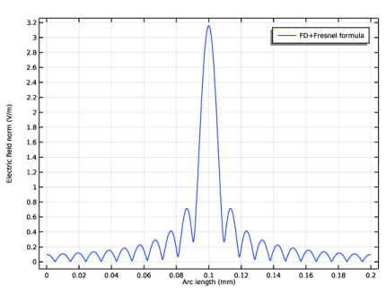
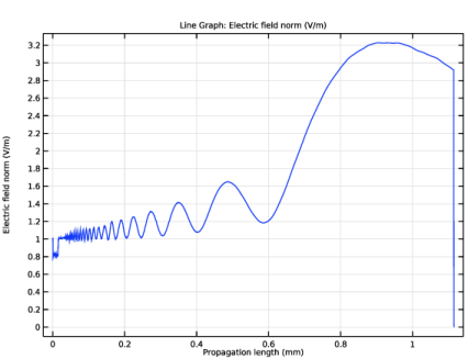
In the associated text field, type Electric field norm (V/m).

Line Graph 1

Right-click and choose .

In the window for , locate the section.

From the list, choose .

Type the expression for the Fresnel diffraction formula.

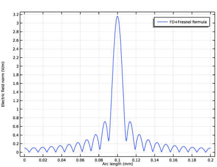
Locate the section. In the text field, type 3/2.5*sqrt(1/wl/f*intop1(ewfd.Ez*exp(-i*k*y^2/(2*f))*exp(i*2*pi*dest(u)*y/(wl*f)))*conj(intop1(ewfd.Ez*exp(-i*k*y^2/(2*f))*exp(i*2*pi*dest(u)*y/(wl*f))))).

Click to expand the section. Select the check box.

From the list, choose .

In the table, enter the following settings:


Legends
FD+Fresnel formula

In the toolbar, click

Add Physics

In the second part of this model, the Electromagnetic Waves, Beam Envelopes interface analyzes the entire domain.

In the toolbar, click

to open the window.

Go to the window.

In the tree, select .

Click in the window toolbar.

In the toolbar, click

to close the window.

Definitions

Perfectly Matched Layer 1 (pml1)

In the toolbar, click

In the window for , locate the section.

From the list, choose .

Electromagnetic Waves, Beam Envelopes (ewbe)

In the window, under click .

In the window for , locate the section.

From the list, choose .

Locate the section. From the list, choose .

Specify the k1 vector as


k*n	x
0	y

Matched Boundary Condition 1

In the toolbar, click

and choose .

In the window for , locate the section.

From the list, choose .

Locate the section. From the list, choose .

Specify the E0 vector as


0	x
0	y
1[V/m]*(abs(y)<w)	z

Transition Boundary Condition 1

Also for this physics interface, add a Transition boundary condition to represent the AR coating on the lens surface.

In the toolbar, click

and choose .

In the window for , locate the section.

From the list, choose .

Locate the section. From the list, choose .

This setting assumes that the wave is incident on the Transition boundary condition boundaries with the wave vector as specified in the section in the settings for the physics interface. This is a slightly better assumption than assuming that the wave propagates in the normal direction to the Transition boundary condition boundaries, which is what the other option represents.