|
|
|

|
1
|
|
2
|
In the Select Physics tree, select Optics>Wave Optics>Electromagnetic Waves, Frequency Domain (ewfd).
|
|
3
|
Click Add.
|
|
4
|
Click
|
|
5
|
|
6
|
Click
|
|
1
|
|
2
|
|
1
|
|
2
|
|
3
|
|
1
|
|
2
|
|
4
|
|
1
|
|
2
|
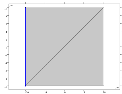
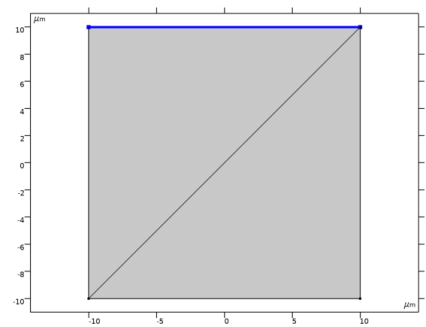
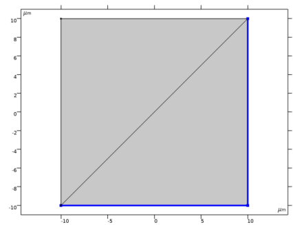
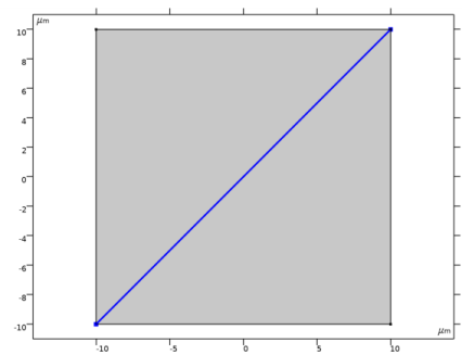
Select the object pol1 only.
|
|
3
|
|
4
|
|
5
|
|
6
|
|
1
|
In the Model Builder window, under Component 1 (comp1) click Electromagnetic Waves, Frequency Domain (ewfd).
|
|
2
|
|
3
|
|
1
|
|
3
|
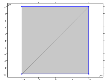
In the Settings window for Scattering Boundary Condition, locate the Scattering Boundary Condition section.
|
|
4
|
|
5
|
|
6
|
|
1
|
|
1
|
|
3
|
In the Settings window for Transition Boundary Condition, locate the Transition Boundary Condition section.
|
|
4
|
|
5
|
|
6
|
|
7
|
|
8
|
|
1
|
|
2
|
|
3
|
|
4
|
|
5
|
|
1
|
|
2
|
|
3
|
|
4
|
|
1
|
|
3
|
|
4
|
|
5
|
|
6
|
|
1
|
|
3
|
|
4
|
|
5
|
|
6
|
|
1
|
|
3
|
|
4
|
|
5
|
|
6
|
|
1
|
|
3
|
|
4
|
|
5
|
|
6
|
|
7
|
|
1
|
|
2
|
|
3
|
|
4
|
|
5
|
|
1
|
|
2
|
|
3
|
|
4
|
|
1
|
Right-click Component 1 (comp1)>Electromagnetic Waves, Beam Envelopes (ewbe) and choose Scattering Boundary Condition.
|
|
3
|
In the Settings window for Scattering Boundary Condition, locate the Scattering Boundary Condition section.
|
|
4
|
|
5
|
|
6
|
|
1
|
|
1
|
|
3
|
In the Settings window for Scattering Boundary Condition, locate the Scattering Boundary Condition section.
|
|
4
|
|
1
|
|
3
|
In the Settings window for Transition Boundary Condition, locate the Transition Boundary Condition section.
|
|
4
|
|
5
|
|
6
|
From the μr list, choose User defined. From the σ list, choose User defined. In the d text field, type 13[nm].
|
|
1
|
|
2
|
|
4
|
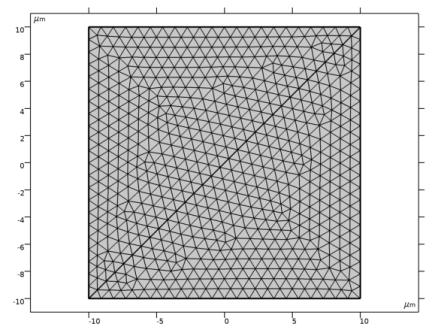
Locate the Electromagnetic Waves, Beam Envelopes (ewbe) section. From the Mesh type list, choose Triangular mesh.
|
|
5
|
|
6
|
|
1
|
|
2
|
|
3
|
|
4
|
|
5
|
|
6
|
|
1
|
|
2
|
|
3
|
|
1
|
|
2
|
|
3
|
|
4
|