Terzaghi Compaction

Fluids that move through pore spaces in an aquifer or reservoir can shield the porous medium from stress because they bear part of the load from, for instance, overlying rocks, sediments, fluids, and buildings. Withdrawing fluids from the pore space increases the stress the solids bear, sometimes to the degree that the reservoir measurably compacts. The reduction in the pore space loops back and alters the fluid pressures. The feedback brings about more fluid movement, and the cycle continues. Terzaghi Compaction describes a conventional flow model and uses the results in postprocessing to calculate vertical compaction following Terzaghi theory (Ref. 2).

Model Definition

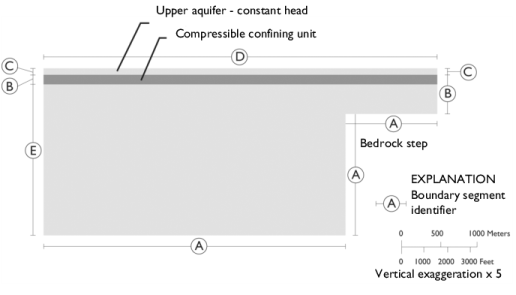
This example analyzes fluid and solid behavior within three sedimentary layers overlying impermeable bedrock in a basin. The bedrock is faulted, which creates a step near a mountain front. The sediment stack totals 420 m at the centerline of the basin (x = 0 m) and thins to 120 m above the step (x > 4000 m). The top two layers are each 20 m thick.

Figure 1: Model geometry showing boundary segments (from Leake and Hsieh, Ref. 1).

Pumping from the lower aquifer reduces hydraulic head down the centerline of the basin by 6 m per year. The head drop moves fluid away from the step. The middle layer is relatively impermeable. The pumping does not diminish the supply of fluids in the unpumped reservoir above it. The flow field is initially at steady state. The period of interest is 10 years.

This example sets up a traditional flow model and analyzes the vertical displacement during postprocessing. The flow field is fully described using the Darcy velocity in an equation of continuity

(1)

where Sh is the storage coefficient (m−1), K equals hydraulic conductivity (m/s), and H represents hydraulic head (m). In most conventional flow models, Sh represents small changes in fluid volume and pore space. It combines terms describing the fluid’s compressibility, the solids’ compressibility, and the reservoir’s porosity. In the original research (Ref. 1) and in this model, Sh is the specific storage of the solid skeleton, Ssk.

Instead of solving Darcy’s law in the hydraulic head formulation, we solve Equation 1 in the pressure formulation

here, the storage coefficient S (1/Pa) is related to the fluid density, acceleration of gravity and the storage coefficient given in Equation 1 by the relation S = Sh/ρg. Also, the hydraulic head is related to the fluid pressure and elevation H = p/ρg + D, and the hydraulic conductivity is related to the permeability and dynamic viscosity of the fluid K = κρg/μ.

Because the aquifer is at equilibrium prior to pumping, you set up this model to predict the change in hydraulic head rather than the hydraulic head values themselves. The main advantage of this approach lies in establishing initial and boundary conditions. Here you specify that the hydraulic head along the centerline of the basin decreases linearly by 60 m over ten years, then simply state that the hydraulic head initially is zero and remains so where heads do not change in time.

The boundary and initial conditions are

where n is the normal to the boundary. The letters A through E, taken from Leake and Hsieh (Ref. 1), denote the boundary (see Figure 1).

Terzaghi theory uses skeletal specific storage or aquifer compressibility to calculate the vertical compaction Δb (m) of the aquifer sediments in a given representative volume as

(2)

where b is standard notation for the vertical thickness of aquifer sediments (m).

Model Data

The following table gives the data for the Terzaghi compaction model:

Table 1: Model Data.
Variable	Description	Value
ρf	Fluid density	1000 kg/m3
Ssk	Skeletal specific storage, aquifer layers	1·10-5 m-1
	Skeletal specific storage, confining layer	1·10-4 m-1
Ks	Hydraulic conductivity, aquifer layers	25 m/d
	Hydraulic conductivity, confining layer	0.01 m/d
H(0)	Initial hydraulic head	0 m
H0(t)	Declining head boundary	(6 m/year)·t

Results and Discussion

Figure 2 shows a Year-10 snapshot from the COMSOL Multiphysics solution to the Terzaghi compaction example. The results describe conventional Darcy flow toward the centering of a basin, moving away from a bedrock step (x > 4000 m). The shading represents the change in hydraulic head brought on by pumping at x = 0 m. The streamlines and arrows denote the direction and magnitude of the fluid velocity. The flow goes from vertical near the surface to horizontal at the outlet. Where the sediments thicken at the edge of the step, the hydraulic gradient and the fluid velocities change abruptly.

Figure 2: COMSOL Multiphysics solution to a Terzaghi flow problem. The figure shows change in hydraulic head (surface plot) and fluid velocity (streamlines).

The compaction calculated according to Equation 2 is shown as a contour plot in Figure 3.

Figure 3: Contour plot of the compaction after 10 years.

References

1. S.A. Leake and P.A. Hsieh, Simulation of Deformation of Sediments from Decline of Ground-Water Levels in an Aquifer Underlain by a Bedrock Step, U.S. Geological Survey Open File Report, 97-47, 1997.

2. K. Terzaghi, Theoretical Soil Mechanics, John Wiley & Sons, p. 510, 1943.

Subsurface_Flow_Module/Flow_and_Solid_Deformation/terzaghi_compaction

Modeling Instructions

From the menu, choose .

New

In the window, click

Model Wizard

In the window, click

In the tree, select .

Click .

Click

In the tree, select .

Click

Geometry 1

Rectangle 1 (r1)

In the toolbar, click

In the window for , locate the section.

In the text field, type 5200.

In the text field, type 440.

Locate the section. In the text field, type -440.

Click to expand the section. Select the check box.

Clear the check box.

In the table, enter the following settings:


Layer name	Thickness (m)
Layer 1	20
Layer 2	20

Click

Rectangle 2 (r2)

In the toolbar, click

In the window for , locate the section.

In the text field, type 1200.

In the text field, type 320.

Locate the section. In the text field, type 4000.

In the text field, type -440.

Click

Click the

button in the toolbar.

Difference 1 (dif1)

In the toolbar, click

and choose .

Select the object only, to add it to the list.

In the window for , locate the section.

Find the subsection. Select the

toggle button.

Select the object only.

In the toolbar, click

Definitions

Because the model geometry is so elongated, you get a better view of it by turning off the default setting that preserves the aspect ratio.

In the window, expand the node.

Axis

In the window, expand the node, then click .

In the window for , locate the section.

From the list, choose .

Click

Now, define variables for the skeletal specific storage and saturated hydraulic conductivity. Using local variables allows you to define variables on different domains with different expressions but identical names.

Variables 1

In the toolbar, click

and choose .

In the window for , locate the section.

From the list, choose .

Select Domains 1 and 3 only.

Locate the section. In the table, enter the following settings:


Name	Expression	Unit	Description
S_sk	1e-5[m^-1]	1/m	Skeletal specific storage
K_s	25[m/day]	m/s	Saturated hydraulic conductivity

Variables 2

In the toolbar, click

and choose .

In the window for , locate the section.

From the list, choose .

Select Domain 2 only.

Locate the section. In the table, enter the following settings:


Name	Expression	Unit	Description
S_sk	1e-4[m^-1]	1/m	Skeletal specific storage
K_s	0.01[m/day]	m/s	Saturated hydraulic conductivity

Materials

Define blank materials and assign them to the domains. Later, after the physics is set up correctly, the materials indicate which material properties are required to solve the problem.

Fluid

In the window, under right-click and choose .

In the window for , type Fluid in the text field.

Porous 1

Right-click and choose .

In the window for , type Porous 1 in the text field.

Locate the section. From the list, choose .

Porous 2

Right-click and choose .

In the window for , type Porous 2 in the text field.

Select Domain 2 only.

Darcy’s Law (dl)

Define all physical effects. After that, the material properties can be completed.

In the window, under click .

In the window for , locate the section.

Select the check box.

Gravity 1

In the window, under click .

In the window for , locate the section.

From the list, choose .

Storage Model 1

In the toolbar, click

and choose .

In the window for , locate the section.

From the list, choose .

Locate the section. From the list, choose .

In the K text field, type K_s.

Locate the section. From the list, choose . In the S text field, type S_sk/dl.rho/g_const.

Locate the section. From the list, choose .

Fill in the missing material properties.

Materials

Fluid (mat1)

In the window, under click .

In the window for , locate the section.

In the table, enter the following settings:


Property	Variable	Value	Unit	Property group
Density	rho	1000	kg/m³	Basic

Porous 1 (mat2)

In the window, click .

In the window for , locate the section.

In the table, enter the following settings:


Property	Variable	Value	Unit	Property group
Porosity	epsilon	0.25	1	Basic

Porous 2 (mat3)

In the window, click .

In the window for , locate the section.

In the table, enter the following settings:


Property	Variable	Value	Unit	Property group
Porosity	epsilon	0.025	1	Basic

Now, set up the boundary conditions.

Darcy’s Law (dl)

Hydraulic Head 1

In the toolbar, click

and choose .

Select Boundary 1 only.

In the window for , locate the section.

In the H0 text field, type -6[m/year]*t.

Hydraulic Head 2

In the toolbar, click

and choose .

Select Boundaries 5, 7, and 12 only.

To calculate the compaction according to Equation 2 first, define a projection operator to integrate along the y-axis. Add a new variable which uses the projection operator to perform a convolution integral using the dest operator.

Definitions

General Projection 1 (genproj1)

In the toolbar, click