|
|
|
|
0.96·10-3 Pa·s
|
|
|
0.954·10-3 Pa·s
|
|
1
|
|
2
|
In the Select Physics tree, select Fluid Flow>Porous Media and Subsurface Flow>Multiphase Flow in Porous Media.
|
|
3
|
Click Add.
|
|
4
|
|
5
|
Click Add.
|
|
6
|
|
7
|
In the Volume fractions table, enter the following settings:
|
|
8
|
|
9
|
|
10
|
|
11
|
|
12
|
In the Dependent variables table, enter the following settings:
|
|
13
|
Click
|
|
14
|
|
15
|
Click
|
|
1
|
|
2
|
|
3
|
|
4
|
|
5
|
|
6
|
|
7
|
Select the Top check box.
|
|
1
|
|
2
|
|
3
|
|
4
|
|
1
|
|
2
|
|
3
|
|
4
|
|
1
|
|
2
|
|
3
|
|
4
|
|
1
|
|
2
|
|
1
|
|
2
|
|
3
|
|
4
|
Browse to the model’s Application Libraries folder and double-click the file reservoir_horizontal_wells_parameters.txt.
|
|
1
|
|
2
|
|
3
|
|
4
|
Browse to the model’s Application Libraries folder and double-click the file reservoir_horizontal_wells_krw.txt.
|
|
5
|
|
6
|
Locate the Interpolation and Extrapolation section. From the Interpolation list, choose Piecewise cubic.
|
|
1
|
|
2
|
|
3
|
|
4
|
Browse to the model’s Application Libraries folder and double-click the file reservoir_horizontal_wells_krn.txt.
|
|
5
|
|
6
|
Locate the Interpolation and Extrapolation section. From the Interpolation list, choose Piecewise cubic.
|
|
1
|
|
2
|
|
3
|
|
4
|
Browse to the model’s Application Libraries folder and double-click the file reservoir_horizontal_wells_pc.txt.
|
|
5
|
|
6
|
Locate the Interpolation and Extrapolation section. From the Interpolation list, choose Piecewise cubic.
|
|
1
|
|
2
|
|
3
|
|
4
|
|
1
|
In the Model Builder window, under Component 1 (comp1) click Phase Transport in Porous Media (phtr).
|
|
2
|
|
3
|
|
1
|
In the Model Builder window, under Component 1 (comp1)>Phase Transport in Porous Media (phtr) click Phase and Porous Media Transport Properties 1.
|
|
2
|
In the Settings window for Phase and Porous Media Transport Properties, locate the Capillary Pressure section.
|
|
3
|
|
4
|
Locate the Phase 1 Properties section. From the ρsw list, choose User defined. In the associated text field, type rhow.
|
|
5
|
|
6
|
|
7
|
Locate the Phase 2 Properties section. From the ρsn list, choose User defined. In the associated text field, type rhoo.
|
|
8
|
|
9
|
|
1
|
|
3
|
|
4
|
|
1
|
|
3
|
|
4
|
|
1
|
|
3
|
|
4
|
|
1
|
|
3
|
|
4
|
|
1
|
|
3
|
|
4
|
|
1
|
|
3
|
|
4
|
|
5
|
|
1
|
|
2
|
|
3
|
|
1
|
In the Model Builder window, under Component 1 (comp1)>Darcy’s Law (dl) click Fluid and Matrix Properties 1.
|
|
2
|
|
3
|
|
4
|
|
5
|
In the κ table, enter the following settings:
|
|
1
|
|
2
|
|
3
|
|
1
|
|
3
|
|
4
|
|
1
|
|
3
|
|
4
|
|
1
|
|
2
|
|
3
|
|
5
|
|
6
|
In the Dependent variable quantity table, enter the following settings:
|
|
7
|
In the Source term quantity table, enter the following settings:
|
|
8
|
|
9
|
|
1
|
In the Model Builder window, under Component 1 (comp1)>Edge ODEs and DAEs (eode) click Distributed ODE 1.
|
|
2
|
|
3
|
|
4
|
|
1
|
|
2
|
|
3
|
|
1
|
|
2
|
|
3
|
|
1
|
|
2
|
|
3
|
|
4
|
|
5
|
|
6
|
Click OK.
|
|
7
|
|
8
|
Click the Custom button.
|
|
9
|
|
11
|
|
12
|
|
13
|
|
1
|
|
2
|
|
3
|
|
4
|
|
5
|
|
6
|
Click OK.
|
|
7
|
|
8
|
|
1
|
|
2
|
|
3
|
|
4
|
|
5
|
|
6
|
Click OK.
|
|
7
|
|
8
|
|
9
|
|
1
|
|
2
|
|
3
|
|
4
|
|
1
|
|
2
|
|
3
|
|
4
|
|
5
|
In the Model Builder window, expand the Study 1>Solver Configurations>Solution 1 (sol1)>Time-Dependent Solver 1 node.
|
|
6
|
|
7
|
|
8
|
|
9
|
Click
|
|
1
|
|
2
|
|
1
|
|
2
|
|
3
|
|
4
|
|
5
|
|
6
|
|
7
|
|
1
|
|
2
|
|
3
|
|
4
|
|
1
|
|
2
|
|
1
|
|
2
|
|
1
|
|
2
|
|
3
|
|
4
|
|
5
|
|
6
|
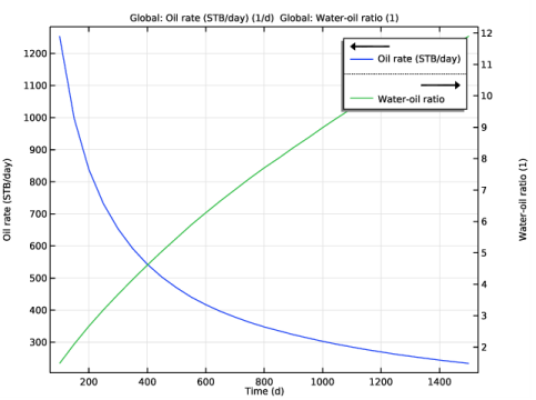
In the associated text field, type Oil rate (STB/day).
|
|
7
|