PDF

Phase Change
Introduction
This example demonstrates how to model a phase change and predicts its impact on a heat transfer analysis. When a material changes phase, for instance from solid to liquid, energy is added to the solid. Instead of creating a temperature rise, the energy alters the material’s molecular structure. Heat consumed or released by a phase change affects fluid flow, magma movement and production, chemical reactions, mineral stability, and many other earth-science applications.
Figure 1: Material properties as functions of temperature.
This 1D example uses the Phase Change Material subfeature from the Heat Transfer Module to examine transient temperature transfer in a rod of ice that heats up and changes to water. In particular, the model demonstrates how to handle material properties that vary as a function of temperature.
This model proceeds as follows. First, estimate the ice-to-water phase change using the transient conduction equation with the latent heat of fusion. Next, compare the first solution to estimates that neglect latent heat. Finally, run additional simulations to evaluate impacts of the temperature interval over which the phase change occurs.
Model Definition
This example describes the ice-to-water phase change along a 1-cm rod of ice. At its left end the rod is insulated, and at the other temperature is maintained at 80 °C. Values for thermal properties depend on the phase. They are presented in Table 1, at 265 K for ice and 300 K for water.
The latent heat of fusion, lm, is 333.5 kJ/kg and the rod is initially at –20 °C.
During the ice-to-water phase change, the density is modified, resulting in a volume compression. The material coordinates express all transformations in the initial coordinate system, when ice occupies all the domain. Assuming that there is no mixing in the liquid phase, the conduction equation in material coordinates can be used. It simplifies the model since you do not need to calculate the velocity field resulting from density variations during phase change. The conduction equation in material coordinates reads
(1)
where ρ (kg/m3) is the density, Ceq (J/kg·K) is the effective heat capacity at constant pressure, keq is the effective thermal conductivity (W/m·K), T is temperature (K), and Q is a heat source (W/m3).
The material properties ρ and keq of water must be in material coordinates. Because values given in Table 1 come from measurements, they correspond to spatial coordinates. Hence, conversion into material coordinates is necessary. In 1D models, you just have to multiply by the ratio of densities, ρratio:
Note: With this transformation, the density of water, ρ, in material coordinates is ρ = ρwaterρratio = ρice. This is consistent with conservation of mass because the integral of ρ over the geometry domain remains constant in time.
The boundary conditions for this model are
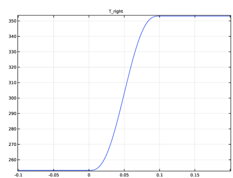
fixed temperature at x = 0.01; the fixed temperature creates a temperature discontinuity at the start time. You can thus replace Thot by a smoothed step function Tright that increases the temperature from T0 to Thot in 0.1 s.
Results and Discussion
Figure 2 shows images of the temperature distribution in time, predicted with latent heat. The system is solid ice at t = 0, and water content increases with time.
Figure 2: Temperature estimates with latent heat at t = 0 s, 15 s, 30 s, 45 s, 60 s, 2 min, 3 min, 4 min, …, 20 min.
The distributions all level out around the 0 °C temperature point because not all of the energy is going toward a temperature rise; some is being absorbed to change the molecular structure and change the phase.
The solution in Figure 3 shows temperature estimates for the simulation without latent heat.
Figure 3: Temperature estimates without latent heat at t = 0  s, 15 s, 30 s, 45 s, 60 s, 2 min, 3 min, 4 min, …, 20 min.
A change of profile also occurs at 0 °C but is less visible. Because latent heat is not accounted for, this change is here due to the different thermophysical properties of water below and above 0 °C.
Figure 4 shows results for different solid-to-liquid intervals at three times. The smaller the interval, the sharper the bend in the temperature profile at zero temperature, T. In the simulations, narrowing the temperature interval to a step change, for example, comes at a large computational cost. In the figure, the results for the wide and narrow pulses compare closely.
Figure 4: Temperature estimates for different temperature intervals for latent heat consumption. Estimates are for dT intervals of 0.5 K (blue), 1 K (green), and 2 K (red) at t = 30 s (three curves at bottom), 5 min (three curves at middle), and 10 min (three curves on top).
References
1. S.E. Ingebritsen and W.E. Sanford, Groundwater in Geologic Processes, Cambridge University Press, 1998.
2. N.H. Sleep and K. Fujita, Principles of Geophysics, Blackwell Science, 1997.
3. D.L. Turcotte and G. Schubert, Geodynamics: Applications of Continuum Physics to Geological Problems, 2nd ed., Cambridge University Press, 2002.
Application Library path: Subsurface_Flow_Module/Heat_Transfer/phase_change
Modeling Instructions
From the File menu, choose New.
New
In the New window, click  Model Wizard.
Model Wizard
1
In the Model Wizard window, click  1D.
2
In the Select Physics tree, select Heat Transfer>Heat Transfer in Fluids (ht).
The Heat Transfer in Fluids interface with its Fluid feature together with the Phase Change Material subfeature solves for the temperature and automatically calculates the equivalent conductivity and the equivalent specific heat capacity.
3
Click Add.
4
Click  Study.
5
In the Select Study tree, select General Studies>Time Dependent.
6
Geometry 1
Interval 1 (i1)
1
In the Model Builder window, under Component 1 (comp1) right-click Geometry 1 and choose Interval.
2
In the Settings window for Interval, locate the Interval section.
3
4
Click  Build Selected.
Form Union (fin)
1
In the Model Builder window, click Form Union (fin).
2
In the Settings window for Form Union/Assembly, click  Build Selected.
3
Click the  Zoom Extents button in the Graphics toolbar.
Global Definitions
The following steps describe how the model parameters are defined.
Parameters 1
1
In the Model Builder window, under Global Definitions click Parameters 1.
2
In the Settings window for Parameters, locate the Parameters section.
3
Step 1 (step1)
1
In the Home toolbar, click  Functions and choose Global>Step.
2
In the Settings window for Step, type T_right in the Function name text field.
3
Locate the Parameters section. In the Location text field, type 0.05.
4
In the From text field, type T_0.
5
In the To text field, type T_hot.
6
Click to expand the Smoothing section. Click  Plot.
Materials
Ice
1
In the Materials toolbar, click  Blank Material.
2
In the Settings window for Material, type Ice in the Label text field.
3
Locate the Material Contents section. In the table, enter the following settings:
Water
1
In the Materials toolbar, click  Blank Material.
2
In the Settings window for Material, type Water in the Label text field.
3
Because the model is solved in material coordinates, the water density and thermal conductivity are converted.
4
Locate the Material Contents section. In the table, enter the following settings:
Heat Transfer in Fluids (ht)
Fluid 1
In the Model Builder window, under Component 1 (comp1)>Heat Transfer in Fluids (ht) click Fluid 1.
Phase Change Material 1
1
In the Physics toolbar, click  Attributes and choose Phase Change Material.
2
In the Settings window for Phase Change Material, locate the Phase Change section.
3
In the ΔT12 text field, type dT.
4
In the L12 text field, type lm.
5
Locate the Phase 1 section. From the Material, phase 1 list, choose Ice (mat1).
6
Locate the Phase 2 section. From the Material, phase 2 list, choose Water (mat2).
Initial Values 1
1
In the Model Builder window, click Initial Values 1.
2
In the Settings window for Initial Values, locate the Initial Values section.
3
In the T text field, type T_0.
Temperature 1
1
In the Physics toolbar, click  Boundaries and choose Temperature.
2
3
In the Settings window for Temperature, locate the Temperature section.
4
In the T0 text field, type T_right(t[1/s]).
Mesh 1
Follow the steps below to generate a relatively fine mesh of 120 elements.
Edge 1
In the Mesh toolbar, click  Edge.
Distribution 1
1
Right-click Edge 1 and choose Distribution.
2
In the Settings window for Distribution, locate the Distribution section.
3
In the Number of elements text field, type 120.
4
Click  Build Selected.
Study 1
Step 1: Time Dependent
1
In the Model Builder window, under Study 1 click Step 1: Time Dependent.
2
In the Settings window for Time Dependent, locate the Study Settings section.
3
Click  Range.
4
In the Range dialog box, type 15 in the Step text field.
5
In the Stop text field, type 60.
6
Click Replace.
7
In the Settings window for Time Dependent, locate the Study Settings section.
8
Click  Range.
9
In the Range dialog box, type 120 in the Start text field.
10
In the Step text field, type 60.
11
In the Stop text field, type 1200.
12
Click Add.
For more robust convergence, tighten the relative tolerance, which controls the size of the time steps taken by the solver.
13
In the Settings window for Time Dependent, locate the Study Settings section.
14
From the Tolerance list, choose User controlled.
15
In the Relative tolerance text field, type 1e-3.
16
In the Home toolbar, click  Compute.
Results
Temperature (ht)
All the parameter values in this model have a time unit of seconds, so the output time you enter here gives a total simulation time of 20 minutes. Different output intervals can be generated by adding other range commands as it is done above. Within the first minute, solution data is stored every 15 seconds, whereas for the remaining simulation period, the data is only stored every 60 seconds.
A line plot of the temperature distribution along the rod for all times is automatically produced. To generate Figure 2, you only need to change the temperature unit.
Line Graph
1
In the Model Builder window, expand the Temperature (ht) node, then click Line Graph.
2
In the Settings window for Line Graph, locate the y-Axis Data section.
3
From the Unit list, choose degC.
4
In the Temperature (ht) toolbar, click  Plot.
Phase Change Without Latent Heat
To analyze the impact of the latent heat terms on the phase change model, a parametric sweep with a single value is used to set the latent heat to 0 in a new study.
Add Study
1
In the Home toolbar, click  Add Study to open the Add Study window.
2
Go to the Add Study window.
3
Find the Studies subsection. In the Select Study tree, select General Studies>Time Dependent.
4
Click Add Study in the window toolbar.
5
In the Home toolbar, click  Add Study to close the Add Study window.
Study 2
Step 1: Time Dependent
1
In the Settings window for Time Dependent, locate the Study Settings section.
2
Click  Range.
3
In the Range dialog box, type 60 in the Stop text field.
4
In the Step text field, type 15.
5
Click Replace.
6
In the Settings window for Time Dependent, locate the Study Settings section.
7
Click  Range.
8
In the Range dialog box, type 120 in the Start text field.
9
In the Stop text field, type 1200.
10
In the Step text field, type 60.
11
Click Add.
12
In the Settings window for Time Dependent, locate the Study Settings section.
13
From the Tolerance list, choose User controlled.
14
In the Relative tolerance text field, type 1e-3.
15
In the Model Builder window, click Step 1: Time Dependent.
16
Click to expand the Study Extensions section. Select the Auxiliary sweep check box.
17
18
19
In the Home toolbar, click  Compute.
Results
Temperature, No Latent Heat
In the Settings window for 1D Plot Group, type Temperature, No Latent Heat in the Label text field.
To generate Figure 3, you only need to change the units in the automatically generated temperature plot.
Line Graph
1
In the Model Builder window, expand the Temperature, No Latent Heat node, then click Line Graph.
2
In the Settings window for Line Graph, locate the y-Axis Data section.
3
From the Unit list, choose degC.
4
In the Temperature, No Latent Heat toolbar, click  Plot.
To be able to keep track of the different studies, rename the datasets containing the solutions of Study 1 and Study 2.
Solution 1, lm Included
1
In the Model Builder window, expand the Results>Datasets node, then click Study 1/Solution 1 (sol1).
2
In the Settings window for Solution, type Solution 1, lm Included in the Label text field.
Solution 2, lm Excluded
1
In the Model Builder window, under Results>Datasets click Study 2/Solution 2 (sol2).
2
In the Settings window for Solution, type Solution 2, lm Excluded in the Label text field.
Phase Change for Varying Transition Intervals
Solutions to the phase change problem vary with the range in temperatures dT over which you assume that the phase transition occurs. To visualize the impact of different transition widths sample results from the original simulation and compare those estimates to results from simulations with varying dT values.
Add Study
1
In the Home toolbar, click  Add Study to open the Add Study window.
2
Go to the Add Study window.
3
Find the Studies subsection. In the Select Study tree, select General Studies>Time Dependent.
4
Click Add Study in the window toolbar.
5
In the Home toolbar, click  Add Study to close the Add Study window.
Study 3
Step 1: Time Dependent
1
In the Settings window for Time Dependent, locate the Study Settings section.
2
Click  Range.
3
In the Range dialog box, type 60 in the Stop text field.
4
In the Step text field, type 15.
5
Click Replace.
6
In the Settings window for Time Dependent, locate the Study Settings section.
7
Click  Range.
8
In the Range dialog box, type 120 in the Start text field.
9
In the Stop text field, type 1200.
10
In the Step text field, type 60.
11
Click Add.
12
In the Settings window for Time Dependent, locate the Study Settings section.
13
From the Tolerance list, choose User controlled.
14
In the Relative tolerance text field, type 1e-3.
Follow the steps below to calculate the temperature distribution of the rod for different values of the transition interval by just adding a parametric sweep to the study node. In this example, use the values 0.1 K, 0.5 K, and 2.5 K for dT.
Parametric Sweep
1
In the Study toolbar, click  Parametric Sweep.
2
In the Settings window for Parametric Sweep, locate the Study Settings section.
3
4
5
In the Study toolbar, click  Compute.
Results
Temperature (ht) 1
Again, the temperature distribution along the rod for all time steps and dT-values is produced automatically. You can modify this plot to generate Figure 4 by following the steps below.
1
In the Settings window for 1D Plot Group, click to expand the Title section.
2
From the Title type list, choose Manual.
3
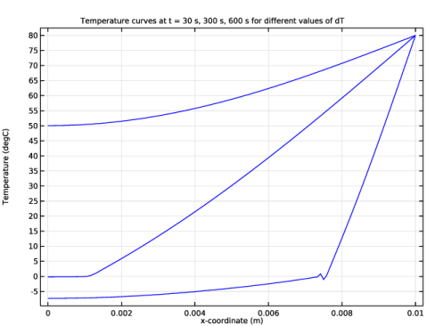
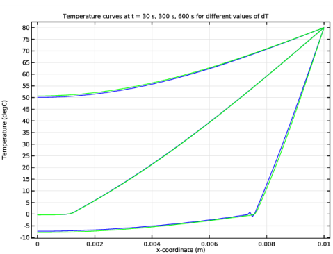
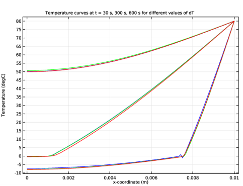
In the Title text area, type Temperature curves at t = 30 s, 300 s, 600 s for different values of dT.
Line Graph
1
In the Model Builder window, expand the Temperature (ht) 1 node, then click Line Graph.
2
In the Settings window for Line Graph, locate the Data section.
3
From the Dataset list, choose Study 3/Parametric Solutions 1 (sol4).
4
From the Parameter selection (dT) list, choose First.
5
From the Time selection list, choose Interpolated.
6
In the Times (s) text field, type 30 300 600.
7
Locate the y-Axis Data section. From the Unit list, choose degC.
8
Click to expand the Coloring and Style section. From the Color list, choose Blue.
9
In the Temperature (ht) 1 toolbar, click  Plot.
Line Graph 2
1
Right-click Line Graph and choose Duplicate.
2
In the Settings window for Line Graph, locate the Data section.
3
From the Parameter selection (dT) list, choose From list.
4
In the Parameter values (dT (K)) list, select 1.
5
Locate the Coloring and Style section. From the Color list, choose Green.
6
In the Temperature (ht) 1 toolbar, click  Plot.
Line Graph 3
1
Right-click Line Graph and choose Duplicate.
2
In the Settings window for Line Graph, locate the Data section.
3
From the Parameter selection (dT) list, choose Last.
4
Locate the Coloring and Style section. From the Color list, choose Red.
5
In the Temperature (ht) 1 toolbar, click  Plot.
Temperature, Varying dT
1
In the Model Builder window, under Results click Temperature (ht) 1.
2
In the Settings window for 1D Plot Group, type Temperature, Varying dT in the Label text field.