PDF

Flow in a Fractured Reservoir
Introduction
This model shows how to set up a simulation of flow through a fractured reservoir. The reservoir includes a discrete fracture network (DFN), where the fractures have a randomized distribution of position, size, orientation and aperture. The model uses the Discrete Fracture Network add-in to create randomized fractures in an existing geometry.
Model Definition
The model geometry is depicted in Figure 1.
Figure 1: Model geometry.
The fracture network in the middle layer is created using the Discrete Fracture Network — 3D add-in. It serves as an example of how to use the add-in. The fracture positions follow a uniform random distribution function, their sizes follow a power-law distribution function, and their orientations follow a Fisher distribution. Details about these distribution functions can be found in the documentation of the add-in. The model is designed in such a way that the results are always identical provided that you follow the instructions. The DFN is reproducible because the same random seed is used for all distributions. The individual steps can nevertheless be applied to basically any DFN. Since the add-in can be used to create DFNs of any complexity, which places high demands on the processing of the geometry, it is recommended to use the CAD kernel, which is why this is also the case here.
Beside the geometry, the add-in also generates variables for the aperture df (m) of the fractures and uses them in a fracture flow feature according to the cubic law. It defines the fracture permeabilty as
with ff being the fracture’s friction factor. The flow is driven by the gradient of the pressure (Pa) only, which is described by Darcy’s law
together with mass conservation
with κ (m2) being the porous matrix permeability, and μ (Pa·s) and ρ (kg/m3) the dynamic viscosity and density of water, respectively. In the fractures, the tangential form of Darcy’s Law is the governing equation.
From above, the reservoir is fed by a precipitation rate and in the lower layer there is a slow flow through a slight gradient in the hydraulic head.
Results and Discussion
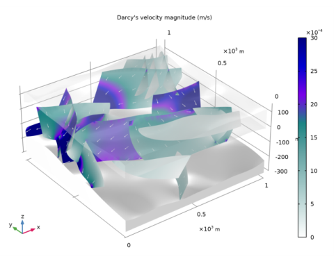
The resulting velocity distribution is shown in Figure 2. Comparing the velocity inside the porous matrix with the velocity field inside the fractures shows that the flow mainly occurs through the fractures.
Figure 2: Velocity distribution in the reservoir.
Application Library path: Subsurface_Flow_Module/Fluid_Flow/fractured_reservoir_flow
Modeling Instructions
From the File menu, choose New.
New
In the New window, click  Model Wizard.
Model Wizard
1
In the Model Wizard window, click  3D.
2
In the Select Physics tree, select Fluid Flow>Porous Media and Subsurface Flow>Darcy’s Law (dl).
3
Click Add.
4
Click  Study.
5
In the Select Study tree, select General Studies>Stationary.
6
Geometry 1
1
In the Model Builder window, under Component 1 (comp1) click Geometry 1.
2
In the Settings window for Geometry, locate the Advanced section.
3
From the Geometry representation list, choose CAD kernel.
Using the CAD kernel is recommended for modeling 3D discrete fracture networks.
4
In the Geometry toolbar, click  Insert Sequence.
5
6
In the Geometry toolbar, click  Build All.
For generating a fracture network consisting of fractures that use randomized distribution functions for size, position and orientation, import the Discrete Fracture Network - 3D add-in.
In the Home toolbar, click  Windows and choose Add-in Libraries.
Add-in Libraries
1
In the Add-in Libraries window, click  Done.
2
In the Developer toolbar, click  Add-ins and choose Discrete Fracture Network - 3D>Discrete Fracture Network - 3D.
Global Definitions
Discrete Fracture Network - 3D 1
1
In the Model Builder window, under Global Definitions click Discrete Fracture Network - 3D 1.
2
In the Settings window for Discrete Fracture Network - 3D, locate the General section.
3
In the Number of Fractures text field type 10.
Because a geometry is present the add-in detects its bounding box and uses it per default.
4
In the Settings window for Discrete Fracture Network - 3D, locate the Size section.
5
6
Click the Use random seed check box to get a reproducible size distribution. Whenever the add-in uses these size parameters and this random seed the size distribution and position is identical.
7
In the Settings window for Discrete Fracture Network - 3D, locate the Orientation section.
8
The dispersion coefficient determines the variance around the strike and dip angle. The larger the value, the smaller the deviation from the given angles.
9
Click the Use random seed check box to get a reproducible orientation distribution.
10
In the Settings window for Discrete Fracture Network - 3D, locate the Properties section.
11
In the Proportionality factor text field enter 1e-5.
Geometry 1
1
In the Model Builder window, under Component 1 (comp1) click Geometry 1.
2
Click Add.
3
Click the  Wireframe Rendering button in the Graphics toolbar to get a better view.
The fractures should only cross the middle layer. Modify the geometry sequence manually to satisfy this requirement.
Partition Objects 1 (dfnpar1)
1
In the Model Builder window, under Component 1 (comp1)>Geometry 1 click Partition Objects 1 (dfnpar1).
2
In the Settings window for Partition Objects, locate the Partition Objects section.
3
Find the Objects to partition subsection. Select the  Activate Selection toggle button.
4
In the list, choose spl1(3) and spl1(4).
5
Click  Remove from Selection.
6
Select the object spl1(2) only.
7
Click  Build Selected.
Add another fracture set with different values.
Global Definitions
Discrete Fracture Network - 3D 1
1
In the Model Builder window, under Global Definitions click Discrete Fracture Network - 3D 1.
2
In the Settings window for Discrete Fracture Network - 3D, locate the General section.
3
In the Number of Fractures text field type 6.
4
In the Settings window for Discrete Fracture Network - 3D, locate the Size section.
5
6
In the Settings window for Discrete Fracture Network - 3D, locate the Orientation section.
7
8
9
Click Add to add a second fracture set.
Geometry 1
Again, modify the geometry sequence.
Partition Objects 2 (dfnpar2)
1
In the Model Builder window, under Component 1 (comp1)>Geometry 1 click Partition Objects 2 (dfnpar2).
2
In the Settings window for Partition Objects, locate the Partition Objects section.
3
Find the Objects to partition subsection. Select the  Activate Selection toggle button.
4
In the list, choose spl1(3) and spl1(4).
5
Click  Remove from Selection.
6
Select the object dfnpar1 only.
7
Click  Build Selected.
8
Click the  Go to XY View button in the Graphics toolbar and compare with the image below.
9
Click the  Go to Default View button in the Graphics toolbar to return to the default view.
Next, add the materials. The top and bottom layers consist of a permeable material, whereas the center layer has a comparatively low permeability. The values are specified later after the physics is set up.
Materials
High permeable
1
In the Model Builder window, under Component 1 (comp1) right-click Materials and choose Blank Material.
2
In the Settings window for Material, type High permeable in the Label text field.
Low permeable
1
Right-click Materials and choose Blank Material.
2
In the Settings window for Material, type Low permeable in the Label text field.
3
Locate the Geometric Entity Selection section. From the Selection list, choose Middle.
4
In the Home toolbar, click  Windows and choose Add Material from Library.
Add Material
1
Go to the Add Material window.
2
In the tree, select Built-in>Water, liquid.
3
Click Add to Component in the window toolbar.
Definitions
The surface is exposed to the environment. Create ambient conditions and define a precipitation rate.
Ambient Properties 1 (ampr1)
1
In the Physics toolbar, click  Shared Properties and choose Ambient Properties.
2
In the Settings window for Ambient Properties, locate the Ambient Conditions section.
3
In the P0,amb text field, type 550[mm/a].
Darcy’s Law (dl)
Next, set up the physics. Start with activating gravity. Define the reference position as the lowest point of the reservoir.
1
In the Model Builder window, under Component 1 (comp1) click Darcy’s Law (dl).
2
In the Settings window for Darcy’s Law, locate the Gravity Effects section.
3
Select the Include gravity check box.
Gravity 1
1
In the Model Builder window, under Component 1 (comp1)>Darcy’s Law (dl) click Gravity 1.
2
In the Settings window for Gravity, locate the Gravity section.
3
Select the Specify reference position check box.
4
Specify the rref vector as
Fluid and Matrix Properties 1
1
In the Model Builder window, click Fluid and Matrix Properties 1.
2
In the Settings window for Fluid and Matrix Properties, locate the Fluid Properties section.
3
From the Fluid material list, choose Water, liquid (mat3).
Fluid and Fracture Properties 1
1
In the Model Builder window, expand the Fracture Flow 1 node, then click Fluid and Fracture Properties 1.
2
In the Settings window for Fluid and Fracture Properties, locate the Fluid Properties section.
3
From the Fluid material list, choose Water, liquid (mat3).
Fluid and Fracture Properties 1
1
In the Model Builder window, expand the Component 1 (comp1)>Darcy’s Law (dl)>Fracture Flow 2 node, then click Fluid and Fracture Properties 1.
2
In the Settings window for Fluid and Fracture Properties, locate the Fluid Properties section.
3
From the Fluid material list, choose Water, liquid (mat3).
The add-in automatically created aperture variables under the Definitions node, which are used by the cubic law.
Materials
It remains to set up the missing material properties.
High permeable (mat1)
1
In the Model Builder window, under Component 1 (comp1)>Materials click High permeable (mat1).
2
In the Settings window for Material, locate the Material Contents section.
3
Low permeable (mat2)
1
In the Model Builder window, click Low permeable (mat2).
2
In the Settings window for Material, locate the Material Contents section.
3
Darcy’s Law (dl)
Next, define the boundary conditions.
Precipitation 1
1
In the Physics toolbar, click  Boundaries and choose Precipitation.
2
3
In the Settings window for Precipitation, locate the Precipitation section.
4
From the P0 list, choose Ambient precipitation rate (ampr1).
5
Select the Slope correction check box.
Hydraulic Head 1
1
In the Physics toolbar, click  Boundaries and choose Hydraulic Head.
2
3
In the Settings window for Hydraulic Head, locate the Hydraulic Head section.
4
In the H0 text field, type 0.5[m/km]*x.
Mesh 1
Next, set up the mesh. For discrete fracture networks the mesh may require manual modifications due to the complexity of the geometry. Start by meshing the domain where the fractures are located.
1
In the Model Builder window, under Component 1 (comp1) click Mesh 1.
2
In the Settings window for Mesh, locate the Physics-Controlled Mesh section.
3
From the Element size list, choose Finer.
4
Locate the Mesh Settings section. From the Sequence type list, choose User-controlled mesh.
Free Tetrahedral 1
1
In the Model Builder window, under Component 1 (comp1)>Mesh 1 click Free Tetrahedral 1.
2
In the Settings window for Free Tetrahedral, locate the Domain Selection section.
3
From the Geometric entity level list, choose Domain.
4
From the Selection list, choose Middle.
Size 1
1
Right-click Free Tetrahedral 1 and choose Size.
2
In the Settings window for Size, locate the Element Size section.
3
From the Predefined list, choose Extra fine.
4
Click  Build Selected.
The mesh contains small elements around fine details resulting from the fractures.
Free Tetrahedral 2
1
In the Mesh toolbar, click  Free Tetrahedral.
2
In the Settings window for Free Tetrahedral, click  Build All.
Study 1
1
In the Model Builder window, click Study 1.
2
In the Settings window for Study, locate the Study Settings section.
3
Clear the Generate default plots check box.
4
In the Home toolbar, click  Compute.
Create a new selection first.
Definitions
Fractures
1
In the Definitions toolbar, click  Union.
2
In the Settings window for Union, locate the Geometric Entity Level section.
3
From the Level list, choose Boundary.
4
Locate the Input Entities section. Under Selections to add, click  Add.
5
In the Add dialog box, in the Selections to add list, choose Fracture network (3D Fracture Network 1 1) and Fracture network (3D Fracture Network 2 1).
6
7
In the Settings window for Union, type Fractures in the Label text field.
Results
Volume Average 1
1
In the Model Builder window, expand the Results node.
2
Right-click Results>Derived Values and choose Average>Volume Average.
3
In the Settings window for Volume Average, locate the Selection section.
4
From the Selection list, choose Middle.
5
Locate the Expressions section. In the table, enter the following settings:
6
Click  Evaluate.
The velocity is around 2e-9 m/s.
Surface Average 2
1
In the Results toolbar, click  More Derived Values and choose Average>Surface Average.
2
In the Settings window for Surface Average, locate the Selection section.
3
From the Selection list, choose Fractures.
4
Locate the Expressions section. In the table, enter the following settings:
5
Click  Evaluate (Table 1 - Volume Average 1).
Table
1
Go to the Table window.
The velocity in the fractures is around 1.7mm/s and thus orders of magnitudes larger than in the matrix.
Create the plot of the Darcy velocity field (Figure 2).
Results
Velocity
1
In the Results toolbar, click  3D Plot Group.
2
In the Settings window for 3D Plot Group, type Velocity in the Label text field.
3
Locate the Plot Settings section. Clear the Plot dataset edges check box.
4
Click to expand the Title section. From the Title type list, choose Manual.
5
In the Title text area, type Darcy's velocity magnitude (m/s) .
Surface 1
1
Right-click Velocity and choose Surface.
2
In the Settings window for Surface, locate the Expression section.
3
In the Expression text field, type dl.U.
4
Locate the Coloring and Style section. From the Color table list, choose AuroraAustralis.
5
Click to expand the Range section. Select the Manual color range check box.
6
In the Maximum text field, type 3e-3.
Selection 1
1
Right-click Surface 1 and choose Selection.
2
In the Settings window for Selection, locate the Selection section.
3
From the Selection list, choose Fractures.
Volume 1
1
In the Model Builder window, right-click Velocity and choose Volume.
2
In the Settings window for Volume, locate the Expression section.
3
In the Expression text field, type dl.U.
4
Click to expand the Inherit Style section. From the Plot list, choose Surface 1.
Selection 1
1
Right-click Volume 1 and choose Selection.
2
In the Settings window for Selection, locate the Selection section.
3
From the Selection list, choose Bottom.
Volume 2
In the Model Builder window, under Results>Velocity right-click Volume 1 and choose Duplicate.
Selection 1
1
In the Model Builder window, expand the Volume 2 node, then click Selection 1.
2
In the Settings window for Selection, locate the Selection section.
3
From the Selection list, choose Top.
Transparency 1
1
In the Model Builder window, right-click Volume 2 and choose Transparency.
2
In the Settings window for Transparency, locate the Transparency section.
3
In the Transparency text field, type 0.8.
Arrow Surface 1
In the Model Builder window, right-click Velocity and choose Arrow Surface.
Selection 1
1
In the Model Builder window, right-click Arrow Surface 1 and choose Selection.
2
In the Settings window for Selection, locate the Selection section.
3
From the Selection list, choose Fractures.
Arrow Surface 1
1
In the Model Builder window, click Arrow Surface 1.
2
In the Settings window for Arrow Surface, locate the Coloring and Style section.
3
From the Arrow length list, choose Logarithmic.
4
Select the Scale factor check box.
5
6
From the Color list, choose White.