Buoyancy Flow with Darcy’s Law

Buoyancy Flow with Darcy’s Law — The Elder Problem

Density variations can initiate flow even in a still fluid. In earth systems, density variations can arise from naturally occurring salts, subsurface temperature changes, or migrating pollution. This buoyant or density-driven flow factors into fluid movement in salt-lake systems, saline-disposal basins, dense contaminant and leachate plumes, and geothermal reservoirs, to name just a few.

This example duplicates a benchmark problem for time-dependent buoyant flow in a porous medium. Known as the Elder problem (Ref. 1), it follows a laboratory experiment to study thermal convection. When Voss and Souza (Ref. 2) recast the Elder problem for salt concentrations, it became a benchmark that many researchers (Ref. 8) have used to test a number of variable-density flow codes including SUTRA (Ref. 3) and SEAWAT (Ref. 4).

This application examines the Elder problem for concentrations through a two-way coupling of two physics interfaces: Darcy’s Law and Transport of Diluted Species in Porous Media.

Model Definition

Figure 1: Geometry for modeling the Elder problem with initial conditions and boundary conditions indicated. In this cross section of a water-saturated porous medium, high salt concentrations exist in the top-right region.

In this example (Figure 1) a vertical cross section of a water-saturated porous medium extends 300 m in the x direction and 150 m in the y direction. The material properties are homogeneous and isotropic. A vertical line at x = 300 m represents a symmetry boundary with a mirror image of the cross section extending beyond it. There is no flow across the geometry edges. High salt concentrations exist at the upper boundary (along y = 150 m) from x = 150 m to 300 m. Salt concentration is zero along the lower boundary. The water is initially stationary (with a hydrostatic pressure distribution) and pristine (zero salt concentration). When the density increases near the high-concentration boundary, flow develops. The period of interest is 20 years. According to Ref. 6 and Ref. 7, the length chosen by Elder is close to a critical value that separates downwelling and upwelling plume structures. As a consequence, the problem is particularly sensitive to perturbations.

Fluid Flow

You can describe the fluid flow in this problem using Darcy’s law:

Here, ρ is the water density (kg/m3), t is the time (s), ε is the porosity, and u is the vector of directional seepage rates, also known as the Darcy velocity. The Darcy velocity u depends on the permeability κ (m2), the fluid’s dynamic viscosity μ (Pa·s), the fluid’s pressure p (Pa), and the acceleration of gravity g (m/s2). The gradient of the elevation D (m) indicates the direction of the vertical coordinate, y.

In Elder’s problem, the fluid density depends linearly on the salt concentration, c (mol/m3) according to

Here, c0 and cs are the normalized salt concentrations of pristine and salty water.

The symmetry or zero flow on all boundaries fix only the change in pressure. For a unique solution, you must also specify a reference pressure. In this example, the pressure at the point (0,0) is fixed. With the Darcy’s Law interface, you express all these conditions as

where n is the unit vector normal to the boundary, and p0 is the reference pressure.

Transport of Diluted Species in Porous Media

The governing equation for this problem is the conservative form of the Transport of Diluted Species in Porous Media interface

where DL is the fluid’s diffusion coefficient (m2/d); θs is the fluid’s volume fraction (porosity); c is the salt concentration (mol/m3), and u is the Darcy velocity (m/s).

In Elder’s problem, the contaminant spreads only by advection and molecular diffusion, and the salt concentration is normalized to unit values.

The only contaminant source in the model domain is the salt concentration along the right half of the upper boundary. The vertical edge at x = 300 m is a symmetry boundary. The remaining boundaries have zero flux. The initial concentration is zero. The following equations represent these conditions:

where n is the unit vector normal to the boundary.

Model Data

The example works with the following data:


Parameter	Name	Value
ρ0	Fresh-water density	1000 kg/m3
ρs	Salt-water density	1200 kg/m3
κ	Permeability	0.5 Darcy
μ	Dynamic viscosity	0.001 Pa·s
g	Gravity	9.81 m/s2
ε	Porosity	0.1
τLDL	Molecular diffusion rate	3.56·10-6 m2/s
cs	Salt-water concentration	1 mol/m3
c0	Fresh-water concentration	0 mol/m3
β	Increase of water density due to concentration changes	200 kg/mol

Note that the original set of parameters for the Elder problem gives a global Peclet number equal to

Here, the difference in water density is ρs − ρ0 = β(cs − c0) = 200 kg/m3, and the length scale L is 150 m. This high Peclet number poses extra difficulties to numerical schemes; see for instance Ref. 5 to Ref. 7.

Results and Discussion

The following results come from the COMSOL Multiphysics solution to a benchmark buoyancy problem that is often used for both temperatures (Ref. 1) and concentrations (Ref. 2).

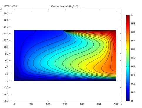
Figure 2 gives snapshots of concentrations at six times during the 20-year simulation period. Initially the water is pristine. By the end of the first year, concentrations spread by diffusion, creating a density gradient. The buoyancy flow begins at the edge of the salt contact, where there is a sharp contrast in fluid density. By the end of year three, the fingering of high concentrations into the reservoir is mature. By year 10, the salt concentrations have spread over roughly 60% of the model domain. The COMSOL Multiphysics solution in Figure 2 is in excellent agreement with that from Elder (Ref. 1).


1 year	10 years
2 years	15 years
3 years	20 years

Figure 2: Snapshots of concentrations from the COMSOL Multiphysics solution to the buoyancy-flow benchmark developed by Voss and Souza (Ref. 2) for the Elder problem.

Figure 3 shows the concentration for the stationary Elder’s problem.

Figure 3: Concentration distribution from the COMSOL Multiphysics solution to the buoyancy-flow benchmark for the stationary Elder problem.

Of interest in the Elder problem is the development of convection cells. The COMSOL Multiphysics plots in Figure 4 reveal the convection cells with the help of velocity streamlines, which the figure shows simultaneously with concentrations for years 3, 10, 15, and 20. At early times, small convection cells develop between the individual fingers of the plume. At late times, a single convection cell covers the model domain.


3 years	15 years
10 years	20 years

Figure 4: Salt concentrations (surface plot) and velocities (streamlines) from the COMSOL Multiphysics solution to a buoyancy benchmark problem (Ref. 2).

This example shows COMSOL Multiphysics applied to a well-known benchmark problem applicable to flow driven by density variations related to either temperature or concentration. The COMSOL Multiphysics results, here for concentration, closely match the benchmark solution (Ref. 2). This buoyant flow is straightforward to set up directly on top of a standard fluid flow and solute-transport model.

References

1. J.W. Elder, “Transient Convection in a Porous Medium”, J. Fluid Mechanics, vol. 27, no. 3, pp. 609–623, 1967.

2. C.I. Voss and W.R. Souza, “Variable Density Flow and Solute Transport Simulation of Regional Aquifers Containing a Narrow Freshwater-saltwater Transition Zone”, Water Resources Research, vol. 23, no. 10, pp. 1851–1866, 1987.

3. C.I. Voss, “A Finite-element Simulation Model for Saturated-unsaturated, Fluid-density-dependent Ground-water Flow with Energy Transport or Chemically-reactive Single-species Solute Transport”, U.S. Geological Survey Water-Resources Investigation Report, 84–4369, 1984.

4. W. Guo and C.D. Langevin, User’s Guide to SEAWAT: A Computer Program for Simulation of Three-Dimensional Variable-Density Ground-Water Flow, U.S. Geological Survey Techniques of Water-Resources Investigations 6-A7, 2002.

5. P. Frolkovic and H. De Schepper, “Numerical modelling of convection dominated transport coupled with density driven flow in porous media”, Advances in Water Resources, vol. 24, no. 1, pp. 63–72, 2000.

6. G.F. Carey, W. Barth, J. A. Woods, B. S. Kirk, M. L. Anderson, S. Chow, and W. Bangerth, “Modelling error and constitutive relations in simulation of flow and transport”, Int. J. Numer. Meth. Fluids, vol. 46, pp. 1211–1236, 2004.

7. J.A. Woods and G.F. Carey, “Upwelling and downwelling behavior in the Elder-Voss-Souza benchmark”, Water Resour. Res., vol. 43, W12403, 2007.

8. J. W. Elder et al “The Elder Problem”, Fluids, vol. 2, p. 11, 2017.

Subsurface_Flow_Module/Solute_Transport/buoyancy_darcy_elder

Modeling Instructions

From the menu, choose .

New

In the window, click

Model Wizard

In the window, click

In the tree, select .

Click .

In the tree, select .

Click .

Click

In the tree, select .

Click

Global Definitions

Parameters 1

In the window, under click .

In the window for , locate the section.

In the table, enter the following settings:


Name	Expression	Value	Description
L	150[m]	150 m	Basin depth
rho0	1000[kg/m^3]	1000 kg/m³	Pristine water density
rho_s	1200[kg/m^3]	1200 kg/m³	Brine density
c0	0[mol/m^3]	0 mol/m³	Zero salt concentration
c_s	1[mol/m^3]	1 mol/m³	Normalized salt concentration
beta	(rho_s-rho0)/(c_s-c0)	200 kg/mol	Increase in density due to salt concentration
p0	0[atm]	0 Pa	Reference pressure
mu	1e-3[Pa*s]	0.001 Pa·s	Dynamic viscosity
kappa	500[mD]	4.9346E-13 m²	Permeability
epsilon	0.1	0.1	Porosity
D_L	3.56e-6[m^2/s]	3.56E-6 m²/s	Molecular diffusion
Pe	beta(c_s-c0)g_constkappaL/(muepsilonD_L)	407.8	Peclet number