Thermal Stress Analysis of a Turbine Stator Blade

PDF

Thermal Stress Analysis of a Turbine Stator Blade

The conditions within gas turbines are extreme. The pressure can be as high as 40 bars, and the temperature far above 1000 K. Any new component must therefore be carefully designed to be able to withstand thermal stress and vibrations due to the rotating machinery and aerodynamic loads exerted by the fluid rushing through the turbine. If a component fails, the high rotational speeds can result in a complete rupture of the whole turbine.

The most extreme conditions are found in the high pressure part downstream of the combustion chamber where hot combustion gas flows through a cascade of rotors and stators. To prevent the parts from melting, relatively “cold” air is taken from bleeding vanes located in the high-pressure compressor casing, then led past the combustion chamber into the turbine casing in order to be used as a coolant. Directly behind the combustion chamber, both internal cooling within ducts and film cooling over the blade side surfaces are applied. Besides, a surface treatment (coating) is often added to the current blades to protect them from hot corrosion. Further downstream, where the temperature is somewhat lower, it may suffice with internal cooling. For more details on gas turbines, see Ref. 1.

Since the physics within a gas turbine is very complex, simplified approaches are often used at the initial stages of the development of the new components. In this tutorial, the thermal stresses in a stator blade with only internal cooling are analyzed (coating and film cooling are not considered).

This application requires the Structural Mechanics Module and the CFD Module or Heat Transfer Module. It also uses the Material Library.

Model Definition

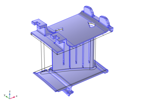
The model geometry is shown in Figure 1. The stator blade profile is a modified version of a design shown in Ref. 2. The model includes some generic mounting details as well as a generic internal cooling duct.

Figure 1: A stator blade with mounting details.

Use the Thermal Stress interface from the Structural Mechanics Module to set up the model. The blade and the mounting details are assumed to be made of the directionally solidified (DS) GTD111 alloy which is a nickel-based alloy with high tensile strength (Ref. 1). This material is available in the COMSOL Material Library. In addition to the data covered by the Material Library, the linear elastic model requires a reference temperature that is set to 300 K and a Poisson’s Ratio that is set to 0.33, a number comparable to that for other stainless steels.

Figure 2 shows the cooling duct. The duct geometry is simplified and does not include details such as the ribs (Ref. 3) typical for cooling ducts. Instead of simulating the complicated flow in the duct, an average Nusselt number correlation from Ref. 3 is used to calculate a heat transfer coefficient. Assume the cooling fluid to be air at 30 bar and 600 K.

Figure 2: The internal cooling duct.

The heat flux on the stator blade surfaces is calculated using the heat transfer coefficient. The pressure and suction sides are approximated as two flat plates using the local heat transfer coefficient for external forced convection. The combustion gases are approximated as air at 30 bar and 1100 K. The corresponding speed of sound is approximately 650 m/s.

Ref. 4 contains a Mach number plot of stators without film cooling. A typical Mach number is 0.45 on the pressure side (the concave side) and 0.7 on the suction side (the convex side). This corresponds to approximately 300 m/s on the pressure side and 450 m/s on the suction side.

The platform walls adjacent to the stator blades are treated in the same way as the stator itself but with the free stream velocity set to 350 m/s.

The stator blade exchanges heat with the cooling air through the boundaries highlighted in Figure 3. It is assumed that the turbine has a local working temperature of 900 K, and that the heat transfer coefficient to the stator is 25 W/(m2·K).

Figure 3: Boundaries through which heat is exchanged with the cooling air.

The attachment of the stator element to a ring support is simulated via roller and spring foundation boundary conditions on a few boundaries. All other boundaries are free to deform as a result of thermal expansion.

Results and Discussion

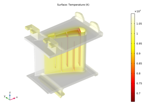
Figure 4 shows a temperature surface plot. The internal cooling creates significant temperature gradients within the blade. However, the trailing edge reaches a temperature close to that of the combustion gases, which indicates that the cooling might be insufficient. The side walls also become very hot, and some additional cooling can be beneficial.

Figure 4: Surface temperature plot.

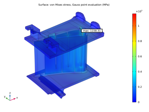
Figure 5 shows a surface plot of the von Mises stress. The maximum stress locally exceeds the yield stress of the material (Ref. 5) in some sharp geometric corners of the internal cooling duct. While this might indicate that the component is at risk for thermal fatigue, no definite assessment can be made without conducting a more advanced analysis that includes a more detailed geometric representation of the duct.

Figure 5: Surface plot of the von Mises stress.

Figure 6: Surface plot of the displacement.

1. M.P. Boyce, Gas Turbine Engineering Handbook, 2nd ed., Gulf Professional Publishing, 2001.

2. NASA, “Power Turbine”, Glenn Research Center, www.grc.nasa.gov/WWW/K-12/airplane/powturb.html.

3. J. Bredberg, “Turbulence Modelling for Internal Cooling of Gas-Turbine Blades”, Thesis for the degree of doctor of philosophy, Chalmers University of Technology, 2002.

4. P. Dahlander, “Source Term Model Approaches to Film Cooling Simulations”, Thesis for the degree of doctor of philosophy, Chalmers University of Technology, 2001.

5. http://www.cnalloys.co.uk/stainless-jethete-m152

Structural_Mechanics_Module/Thermal-Structure_Interaction/turbine_stator

Modeling Instructions

Instructions below require to select entities corresponding to a particular numbers list. For example:
Select Boundaries 113 and 139 only.
In most cases the easiest way to select them is to click the button

and paste the numbers as they are printed in the document (for example paste “113 and 139” for the example above).

From the menu, choose .

In the window, click

.

1

In the window, click

.

2

In the tree, select .

3

4

5

In the tree, select .

6

Global Definitions

1

In the window, under click .

2

In the window for , locate the section.

3

In the table, enter the following settings:


Name	Expression	Value	Description
Pr_cool	0.72	0.72	Cooling Prandtl number
U_suction_side	450[m/s]	450 m/s	Gas velocity on stator suction side
U_pressure_side	300[m/s]	300 m/s	Gas velocity on stator pressure side
U_platform	350[m/s]	350 m/s	Gas velocity along platform walls
T_gas	1100[K]	1100 K	Gas temperature
p_high	30[bar]	3E6 Pa	High pressure level
mu_cool	3.1e-5[Pa*s]	3.1E-5 Pa·s	Viscosity of the cooling air
Cp_cool	770[J/kg/K]	770 J/(kg·K)	Heat capacity of the cooling air
T_cool	600[K]	600 K	Cooling air temperature
H_cool	0.01[m]	0.01 m	Characteristic length scale of cooling channels
T_work	900[K]	900 K	Working temperature
Nu_cool	400	400	Average Nusselt number in cooling channel

Import 1 (imp1)

1

In the toolbar, click

.

2

In the window for , locate the section.

3

4

Browse to the model’s Application Libraries folder and double-click the file turbine_stator.mphbin.

5

To see the interior:

6

button in the toolbar.

The imported geometry should look as shown in the Figure 1.

7

In the toolbar, click

.

8

button in the toolbar.

Define a number of sections to simplify the model setup. First define the internal cooling duct boundaries.

1

In the toolbar, click

.

2

In the window for , type Cooling Duct in the text field.

3

Locate the section. From the list, choose .

4

.

5

In the dialog box, type 222-225, 236, 261-266, 270-271, 278-279, 283-285, 292-305, 308-311, 313-314, 316, 321 in the text field.

If you are reading an electronic version of this document, you can copy the geometric entity numbers from the text.

6

7

button in the toolbar.

8

button in the toolbar.

The selection is shown in Figure 2.

Proceed to select the boundaries through which the heat exchange with the rest of the turbine occurs (Figure 3).

Exchange Boundaries

1

In the toolbar, click

.

2

In the window for , type Exchange Boundaries in the text field.

3

Locate the section. From the list, choose .

4

.

5

In the dialog box, type 3-4, 9, 12, 14, 16, 19-20, 22-24, 28-96, 98-117, 122-135, 138-162, 166-221, 223, 226-231, 239-260, 267-269, 272-277, 280-282, 322-444 in the text field.

6

1

In the toolbar, click

to open the window.

2

Go to the window.

3

In the tree, select .

4

Click in the window toolbar.

5

In the toolbar, click

to close the window.

GTD111 DS [solid,longitudinal] (mat1)

1

In the window for , locate the section.

2

In the table, enter the following settings:


Property	Variable	Value	Unit	Property group
Poisson’s ratio	nu	0.33	1	Young’s modulus and Poisson’s ratio
Thermal conductivity	k_iso ; kii = k_iso, kij = 0	k(T[1/K])[W/(m*K)]	W/(m·K)	Basic

3

In the window, expand the node.

Piecewise (E_solid_longitudinal_1)

1

In the window, expand the node, then click .

2

In the window for , locate the section.

3

From the list, choose .

Thermal Expansion 1 (te1)

1

In the window, under click .

2

In the window for , locate the section.

3

.

Global Definitions

Default Model Inputs

1

In the window, under click .

2

In the window for , locate the section.

3

Find the subsection. In the text field, type 300[K].

Heat Transfer in Solids (ht)

Initial Values 1

1

In the window, under click .

2

In the window for , locate the section.

3

In the T text field, type T_gas.

1

In the toolbar, click

and choose .

2

In the window for , locate the section.

3

From the list, choose .

4

Locate the section. Click the button.

5

In the h text field, type 25.

6

In the Text text field, type T_work.

1

In the toolbar, click

and choose .

2

In the window for , locate the section.

3

From the list, choose .

4

Locate the section. Click the button.

5

In the h text field, type Nu_cool*mu_cool*Cp_cool/2/Pr_cool/H_cool.

6

In the Text text field, type T_cool.

1

In the toolbar, click

and choose .

2

Select Boundaries 137 and 163 only.

3

In the window for , locate the section.

4

Click the button.

5

From the list, choose .

6

From the list, choose .

7

In the xpl text field, type 0.1675-x.

8

In the U text field, type U_suction_side.

9

In the pA text field, type p_high.

10

In the Text text field, type T_gas.

1

In the toolbar, click

and choose .

2

Select Boundaries 136 and 312 only.

3

In the window for , locate the section.

4

Click the button.

5

From the list, choose .

6

From the list, choose .

7

In the xpl text field, type 0.1675-x.

8

In the U text field, type U_pressure_side.

9

In the pA text field, type p_high.

10

In the Text text field, type T_gas.

1

In the toolbar, click

and choose .

2

Select Boundaries 15, 21, 118–121, 164, 165, 232, 234, 235, 237, 286, 289–291, 306, 307, 315, 317, and 320 only.

3

In the window for , locate the section.

4

Click the button.

5

From the list, choose .

6

From the list, choose .

7

In the xpl text field, type 0.19-x.

8

In the U text field, type U_platform.

9

In the pA text field, type p_high.

10

In the Text text field, type T_gas.

Solid Mechanics (solid)

In the window, under click .

1

In the toolbar, click

and choose .

2

Select Boundaries 140, 146, and 213 only.

Spring Foundation 1

1

In the toolbar, click

and choose .

2

Select Boundaries 426 and 428 only.

3

In the window for , locate the section.

4

From the list, choose .

5

In the kA table, enter the following settings:


1e9	0	0
0	0	0
0	0	0

Spring Foundation 2

1

In the toolbar, click

and choose .

2

Select Boundaries 82, 90, 192, and 255 only.

3

In the window for , locate the section.

4

From the list, choose .

5

In the kA table, enter the following settings:


0	0	0
0	0	0
0	0	1e10

Spring Foundation 3

1

In the toolbar, click

and choose .

2

Select Boundary 17 only.

3

In the window for , locate the section.

4

From the list, choose .

5

In the kA table, enter the following settings:


0	0	0
0	1e9	0
0	0	0

In the window, under right-click and choose .

1

In the window for , locate the section.

2

From the list, choose .

1

In the window, click .

2

In the window for , locate the section.

3

From the list, choose .

4

From the list, choose .

5

Locate the section. From the list, choose .

Free Tetrahedral 1

1

In the toolbar, click

.

2

In the window for , click

.

In the toolbar, click

.

The first default plot shows the von Mises stress. Disable the deformation and create a max/min plot to display the critical point in the stator.

1

In the window, expand the node, then click .

2

In the window for , locate the section.

3

In the text field, type solid.misesGp.

4

From the list, choose .

1

In the window, expand the node.

2

Right-click and choose .

1

In the window, right-click and choose .

2

In the window for , locate the section.

3

From the list, choose .

4

Locate the section. From the list, choose .

5

Select the check box.

6

button in the toolbar.

7

button in the toolbar.

The second default plot shows the temperature distribution Figure 4.

Temperature (ht)

1

In the window, click .

2

In the window for , locate the section.

3

Clear the check box.

4

In the toolbar, click

.

5

button in the toolbar.

Finally, plot the displacement (Figure 6).

1

In the toolbar, click

and choose .

2

In the window for , type Displacement in the text field.

1

Right-click and choose .

2

In the window for , click in the upper-right corner of the section. From the menu, choose .

3

Locate the section. From the list, choose .

4

In the toolbar, click

.

5

button in the toolbar.