PDF

Sensitivity Analysis of a Truss Tower
Introduction
Sensitivity analysis is an efficient way of computing the gradient of an objective function with respect to many control variables. In this example, the pitch and yaw in the top of a truss tower are used as objective functions. The sensitivities of these angles to changes in the individual bar diameters are then computed.
Model Definition
The truss geometry consists of a unit cell that is repeated fives times, see Figure 1. The tower is made from structural steel.
Figure 1: The geometry of the tower.
The four points in the bottom are pinned, while the top four points are subjected to two load cases: bending and torsion.
The bending load case is created by subjecting each of the top four points to a force of 10 kN in the x direction.
The torsion load case is created by subjecting the points to a force of 10 kN in the xy-plane, with a direction that is orthogonal to the vector going from the center of the tower to the point.
Using straightforward trigonometry, the tilt and yaw angles are computed by considering the displacement of the top four corners.
Results and Discussion
Figure 2 shows the tilt sensitivity for the bending load case to the left and the torsion load case to the right, respectively. The tower does not tilt in response to torsion, and looking at the color scale one can see that this property is not sensitive to changes in the bar diameters. As one might expect, the lower vertical bars should be reinforced to reduce tilt in response to bending.
Figure 2: The tilt sensitivity of the tower is plotted for both the bending and the torsion load case.
Similarly, Figure 3 shows the yaw sensitivity. The tower does not yaw in response to bending, but it can be made to do so by strengthening and weakening some of the diagonal bars. As one would expect, the diagonal bars (at all heights) are the ones that need higher stiffness to reduce yaw in response to torsion.
Figure 3: The yaw sensitivity of the tower is plotted for both the bending and the torsion load case.
Notes About the COMSOL Implementation
The bar diameters are coupled to the sensitivity analysis by defining a control variable field on all edges. This is then used for the cross-sectional data in the truss interface.
The mast has 134 bars, but in this case the use of adjoint sensitivity doubles the computational cost compared to just solving for the displacement field. This model is linear, but for a nonlinear problem the sensitivity analysis only adds the cost of an extra nonlinear iteration.
Adjoint sensitivity analysis is the foundation of gradient-based optimization. It is supported for stationary (including frequency domain) and transient solvers. For more information, see Theory for the Sensitivity Interface in the Optimization Module User’s Guide.
Application Library path: Structural_Mechanics_Module/Sensitivity_and_Optimization/tower_sensitivity
Modeling Instructions
From the File menu, choose New.
New
In the New window, click  Model Wizard.
Model Wizard
1
In the Model Wizard window, click  3D.
2
In the Select Physics tree, select Structural Mechanics>Truss (truss).
3
Click Add.
4
In the Select Physics tree, select Mathematics>Optimization and Sensitivity>Sensitivity (sens).
5
Click Add.
6
Click  Study.
7
In the Select Study tree, select General Studies>Stationary.
8
Geometry 1
Create the geometry. To simplify this step, insert a prepared geometry sequence.
1
In the Geometry toolbar, click  Insert Sequence.
2
3
In the Geometry toolbar, click  Build All.
4
Click the  Zoom Extents button in the Graphics toolbar.
5
In the Model Builder window, collapse the Geometry 1 node.
Add Material
1
In the Home toolbar, click  Add Material to open the Add Material window.
2
Go to the Add Material window.
3
In the tree, select Built-in>Structural steel.
4
Click Add to Component in the window toolbar.
5
In the Home toolbar, click  Add Material to close the Add Material window.
Component 1 (comp1)
Add a cylindrical coordinate system for imposing the twisting load case.
Definitions
Cylindrical System 2 (sys2)
1
In the Definitions toolbar, click  Coordinate Systems and choose Cylindrical System.
2
In the Settings window for Cylindrical System, locate the Settings section.
3
Find the Origin subsection. In the table, enter the following settings:
Sensitivity (sens)
Control Variable Field 1
1
In the Model Builder window, under Component 1 (comp1) right-click Sensitivity (sens) and choose Edges>Control Variable Field.
2
In the Settings window for Control Variable Field, locate the Edge Selection section.
3
From the Selection list, choose All edges.
4
Locate the Control Variable section. In the Control variable name text field, type Abar.
5
In the Initial value text field, type 1.
6
Locate the Discretization section. From the Shape function type list, choose Discontinuous Lagrange.
7
Find the Base geometry subsection. From the Element order list, choose Constant.
Global Definitions
Parameters 1
Add the diameters of the bars to the list of parameters.
1
In the Model Builder window, under Global Definitions click Parameters 1.
2
In the Settings window for Parameters, locate the Parameters section.
3
Truss (truss)
1
In the Model Builder window, under Component 1 (comp1) click Truss (truss).
2
In the Settings window for Truss, locate the Edge Selection section.
3
From the Selection list, choose Truss Tower.
Cross-Section Data 1
1
In the Model Builder window, under Component 1 (comp1)>Truss (truss) click Cross-Section Data 1.
2
In the Settings window for Cross-Section Data, locate the Cross-Section Data section.
3
In the A text field, type pi/4*d1^2*Abar.
Cross-Section Data 2
1
In the Physics toolbar, click  Edges and choose Cross-Section Data.
2
In the Settings window for Cross-Section Data, locate the Edge Selection section.
3
From the Selection list, choose Non-Vertical Bars.
4
Locate the Cross-Section Data section. In the A text field, type pi/4*d2^2*Abar.
Pinned 1
1
In the Physics toolbar, click  Points and choose Pinned.
2
In the Settings window for Pinned, locate the Point Selection section.
3
From the Selection list, choose Bottom Points.
Point Load 1
1
In the Physics toolbar, click  Points and choose Point Load.
2
In the Settings window for Point Load, locate the Point Selection section.
3
From the Selection list, choose Top Points.
4
Locate the Force section. Specify the FP vector as
5
In the Physics toolbar, click  Load Group and choose New Load Group.
Point Load 2
1
In the Physics toolbar, click  Points and choose Point Load.
2
In the Settings window for Point Load, locate the Point Selection section.
3
From the Selection list, choose Top Points.
4
Locate the Coordinate System Selection section. From the Coordinate system list, choose Cylindrical System 2 (sys2).
5
Locate the Force section. Specify the FP vector as
6
In the Physics toolbar, click  Load Group and choose New Load Group.
Add an Average Rotation feature to compute the tilt and yaw angles of the truss tower.
Average Rotation 1
1
In the Physics toolbar, click  Global and choose Average Rotation.
2
In the Settings window for Average Rotation, locate the Point Selection section.
3
From the Selection list, choose Top Points.
Global Definitions
Load Group: Bending
1
In the Model Builder window, under Global Definitions>Load and Constraint Groups click Load Group 1.
2
In the Settings window for Load Group, type Load Group: Bending in the Label text field.
3
In the Parameter name text field, type Bending.
Load Group: Torsion
1
In the Model Builder window, under Global Definitions>Load and Constraint Groups click Load Group 2.
2
In the Settings window for Load Group, type Load Group: Torsion in the Label text field.
3
In the Parameter name text field, type Torsion.
Tilt Sensitivity
1
In the Model Builder window, click Study 1.
2
In the Settings window for Study, type Tilt Sensitivity in the Label text field.
3
Locate the Study Settings section. Clear the Generate default plots check box.
4
Click the  Show More Options button in the Model Builder toolbar.
5
In the Show More Options dialog box, in the tree, select the check box for the node Study>Sensitivity.
6
Click OK to enable the Sensitivity study step.
Sensitivity
1
In the Study toolbar, click  Sensitivity.
2
In the Settings window for Sensitivity, locate the Objective Function section.
3
Step 1: Stationary
1
In the Model Builder window, click Step 1: Stationary.
2
In the Settings window for Stationary, click to expand the Study Extensions section.
3
Select the Define load cases check box.
4
Click  Add twice.
5
6
In the Study toolbar, click  Compute.
Results
Global Evaluation 1
1
In the Model Builder window, expand the Results node.
2
Right-click Results>Derived Values and choose Global Evaluation.
3
In the Settings window for Global Evaluation, locate the Expressions section.
4
5
Click  Evaluate.
The tower only tilts in response to bending and yaws in response to torsion.
Tilt Sensitivity
1
In the Results toolbar, click  3D Plot Group.
2
In the Settings window for 3D Plot Group, type Tilt Sensitivity in the Label text field.
3
Click to expand the Title section. From the Title type list, choose None.
Line 1
1
Right-click Tilt Sensitivity and choose Line.
2
In the Settings window for Line, locate the Expression section.
3
In the Expression text field, type fsens(Abar).
4
Locate the Coloring and Style section. From the Line type list, choose Tube.
5
Select the Symmetrize color range check box.
6
Click to expand the Quality section. From the Smoothing list, choose Inside geometry domains.
The tower does not tilt in response to torsion and the color scale tells that this property is not sensitive to the bar diameters.
Line 2
1
Right-click Line 1 and choose Duplicate.
2
In the Settings window for Line, locate the Data section.
3
From the Dataset list, choose Tilt Sensitivity/Solution 1 (sol1).
4
From the Load case list, choose Bending.
5
Locate the Coloring and Style section. From the Color table list, choose Cividis.
Deformation 1
1
Right-click Line 2 and choose Deformation.
2
In the Settings window for Deformation, locate the Expression section.
3
In the X component text field, type -4.
4
In the Y component text field, type 0.
5
In the Z component text field, type 0.
6
Locate the Scale section. Select the Scale factor check box.
7
Tilt Sensitivity
In the Model Builder window, click Tilt Sensitivity.
Arrow Point 1
1
In the Tilt Sensitivity toolbar, click  More Plots and choose Arrow Point.
2
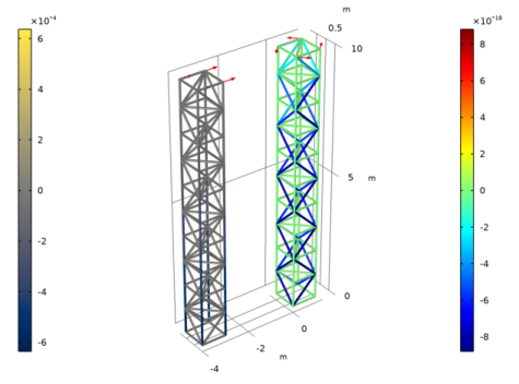
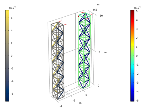
In the Settings window for Arrow Point, click Replace Expression in the upper-right corner of the Expression section. From the menu, choose Component 1 (comp1)>Truss>Load>truss.F_Px,truss.F_Py,truss.F_Pz - Load.
Arrow Point 2
1
Right-click Arrow Point 1 and choose Duplicate.
2
In the Settings window for Arrow Point, locate the Data section.
3
From the Dataset list, choose Tilt Sensitivity/Solution 1 (sol1).
4
From the Load case list, choose Bending.
Deformation 1
1
Right-click Arrow Point 2 and choose Deformation.
2
In the Settings window for Deformation, locate the Expression section.
3
In the X component text field, type -4.
4
In the Y component text field, type 0.
5
In the Z component text field, type 0.
6
Locate the Scale section. Select the Scale factor check box.
7
Tilt Sensitivity
1
In the Model Builder window, click Tilt Sensitivity.
2
In the Settings window for 3D Plot Group, locate the Color Legend section.
3
From the Position list, choose Alternating.
4
Click the  Show Axis Orientation button in the Graphics toolbar.
5
In the Tilt Sensitivity toolbar, click  Plot.
As one might expect, the lower vertical bars should be made stiffer to reduce tilt in response to bending.
Add a new study to investigate the yaw sensitivity.
Add Study
1
In the Home toolbar, click  Add Study to open the Add Study window.
2
Go to the Add Study window.
3
Find the Studies subsection. In the Select Study tree, select General Studies>Stationary.
4
Click Add Study in the window toolbar.
5
In the Home toolbar, click  Add Study to close the Add Study window.
Study 2
Step 1: Stationary
1
In the Settings window for Stationary, locate the Study Extensions section.
2
Select the Define load cases check box.
3
Click  Add twice.
4
5
In the Model Builder window, click Study 2.
6
In the Settings window for Study, type Yaw Sensitivity in the Label text field.
7
Locate the Study Settings section. Clear the Generate default plots check box.
Sensitivity
1
In the Study toolbar, click  Sensitivity.
2
In the Settings window for Sensitivity, locate the Objective Function section.
3
4
In the Study toolbar, click  Compute.
Results
Yaw Sensitivity
1
In the Model Builder window, right-click Tilt Sensitivity and choose Duplicate.
2
In the Settings window for 3D Plot Group, locate the Data section.
3
From the Dataset list, choose Yaw Sensitivity/Solution 2 (sol2).
4
In the Label text field, type Yaw Sensitivity.
Arrow Point 2
1
In the Model Builder window, expand the Yaw Sensitivity node, then click Arrow Point 2.
2
In the Settings window for Arrow Point, locate the Data section.
3
From the Dataset list, choose Yaw Sensitivity/Solution 2 (sol2).
Line 2
1
In the Model Builder window, click Line 2.
2
In the Settings window for Line, locate the Data section.
3
From the Dataset list, choose Yaw Sensitivity/Solution 2 (sol2).
Yaw Sensitivity
1
In the Model Builder window, click Yaw Sensitivity.
2
In the Yaw Sensitivity toolbar, click  Plot.
The tower does not yaw in response to bending, but it is possible to achieve such an effect by stiffening and weakening some of the diagonal bars.
As one would expect, the diagonal bars (at all heights) are the ones that need higher stiffness to reduce yaw in response to torsion.