Instability of a Space Arc Frame

PDF

Instability of a Space Arc Frame

Model Definition

In this example you study the lateral deflection of a space frame subjected to concentrated vertical loading at four different points. A small lateral load is applied to break the symmetry of the structure. The model is described in detail in section 6.3 of Ref. 1, where it is called “Space frame subjected to concentrated loading”. A schematic description of the frame and loads are shown in Figure 1. There are two types of members used in the frame, marked as 1 and 2 respectively.

Figure 1: Space frame geometry.

•

Cross section properties of type 1 members are A1 = 0.5, Iy1 = 0.4, Iz1=0.133.

•

Cross section properties of type 2 members are A2 = 0.1, Iy2 = 0.05, Iz2=0.05.

The local y direction coincides with the global y direction.

The torsional constant is not supplied in the reference, so the common approximation J = Iy + Iz is used.

Linear elastic with E = 4.32·105 and G = 1.66·105.

Constraints and Loads

•

All the base points of the frame are pinned.

•

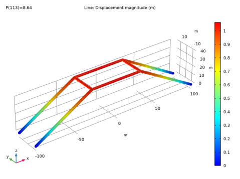
The four corners at the top are subjected to vertical loads P, ranging from 0 to 8.65, acting downward.

•

The front two corners are subjected to lateral loads of 0.001·P.

Results and Discussion

With only vertical loads active on the frame this is a symmetric problem. Hence, it is necessary to perturb the symmetry somewhat to induce a controlled instability. The small lateral loads serve this purpose. As an alternative, you could introduce an initial imperfection in the geometry.

Figure 2 below shows the final state of the frame.

Figure 2: Final state of the deformed frame.

The horizontal displacement of point A on the frame versus the compressive load is shown in Figure 3. Data obtained from Ref. 1 is marked on the same curve. The agreement with the data from the reference is very good.

Figure 3: Load vs. displacement.

The plot of the lateral deflection shows that an instability occurs at a parameter value close to 8.0. In practice, the critical load of an imperfect structure is often significantly lower than that of the ideal structure.

Linear buckling analysis also gives the first critical buckling load as 8.67 which matches well with the critical load obtained from the above analysis. The corresponding buckling mode shape is shown in the Figure 4 below.

Figure 4: First buckling mode.

1. Z.X. Li and L. Vu-Quoc, A Mixed Co-rotational 3D Beam Element for Arbitrarily Large Rotations, Advanced Steel Construction Vol. 6, No. 2, 767-787, 2010.

Structural_Mechanics_Module/Verification_Examples/space_frame_instability

Modeling Instructions

From the menu, choose .

In the window, click

.

1

In the window, click

.

2

In the tree, select .

3

4

5

In the tree, select .

6

Global Definitions

Define the load parameter as well as the geometric data.

1

In the window, under click .

2

In the window for , locate the section.

3

.

4

Browse to the model’s Application Libraries folder and double-click the file space_frame_instability_parameters.txt.

Since the frame is symmetric, create only one quarter of the geometry and use two mirror operations to obtain the full geometry.

Polygon 1 (pol1)

1

In the toolbar, click

and choose .

2

In the window for , locate the section.

3

From the list, choose .

4

In the text field, type -l1-l2/2 -l2/2 -l2/2 0 .

5

In the text field, type -b/2 -b/2 -b/2 -b/2.

6

In the text field, type 0 h1 h1 h1.

Line Segment 1 (ls1)

1

In the toolbar, click

and choose .

2

In the window for , locate the section.

3

From the list, choose .

4

Locate the section. From the list, choose .

5

Locate the section. In the text field, type -l2/2, to -b/2, and to h1.

6

Locate the section. In the text field, type -l2/2 and to h1.

Mirror 1 (mir1)

1

In the toolbar, click

and choose .

2

Click in the window and then press Ctrl+A to select both objects.

3

In the window for , locate the section.

4

Select the check box.

5

Locate the section. In the text field, type -l2/2.

6

In the text field, type h1.

7

Locate the section. In the text field, type 1.

8

In the text field, type 0.

Mirror 2 (mir2)

1

In the toolbar, click

and choose .

2

Click in the window and then press Ctrl+A to select all objects.

3

In the window for , locate the section.

4

Select the check box.

5

Locate the section. In the text field, type 1.

6

In the text field, type 0.

7

In the toolbar, click

.

8

button in the toolbar.

Linear Elastic Material 1

1

In the window, under click .

2

In the window for , locate the section.

3

From the list, choose .

Material 1 (mat1)

1

In the window, under right-click and choose .

2

In the window for , locate the section.

3

In the table, enter the following settings:


Property	Variable	Value	Unit	Property group
Young’s modulus	E	4.32e5	Pa	Basic
Shear modulus	G	1.66e5	N/m²	Bulk modulus and shear modulus
Density	rho	0	kg/m³	Basic

The density is set to zero since it is not used in the present analysis.

Cross-Section Data 1

1

In the window, under click .

2

In the window for , locate the section.

3

In the A text field, type A1.

4

In the Izz text field, type Iz1.

5

In the Iyy text field, type Iy1.

6

In the J text field, type Iy1+Iz1.

Section Orientation 1

1

In the window, click .

2

In the window for , locate the section.

3

From the list, choose .

4

Specify the V vector as


0	X
1	Y
0	Z

Cross-Section Data 2

1

In the toolbar, click

and choose .

2

Select Edges 3, 5, 9, and 11 only.

3

In the window for , locate the section.

4

In the A text field, type A2.

5

In the Izz text field, type Iz2.

6

In the Iyy text field, type Iy2.

7

In the J text field, type Iy2+Iz2.

Section Orientation 1

1

In the window, expand the node, then click .

2

In the window for , locate the section.

3

From the list, choose .

4

Specify the V vector as


1	X
0	Y
0	Z

1

In the toolbar, click

and choose .

2

Select Points 1, 2, 11, and 12 only.

1

In the toolbar, click

and choose .

2

Select Points 3, 5, 8, and 10 only.

3

In the window for , locate the section.

4

Specify the FP vector as


0	x
0	y
-P	z

1

In the toolbar, click

and choose .

2

Select Points 3 and 8 only.

3

In the window for , locate the section.

4

Specify the FP vector as


0	x
0.001*P	y
0	z

1

In the window, under click .

2

In the window for , locate the section.

3

From the list, choose .

Step 1: Stationary

Use geometric nonlinearity since the problem is expected to have an instability.

1

In the window, under click .

2

In the window for , locate the section.

3

Select the check box.

Set up parametric sweep for the load.

4

Click to expand the section. Select the check box.

5

Due to instability, the load increment for >8 is reduced.

6

In the table, enter the following settings:


Parameter name	Parameter value list
P (Load)	range(0,0.1,8) range(8.02, 0.02, 8.65)

Solution 1 (sol1)

1

In the toolbar, click

.

Scale the dependent variables appropriately.

2

In the window, expand the node.

3

In the window, expand the node, then click .

4

In the window for , locate the section.

5

From the list, choose .

6

In the window, click .

7

In the window for , locate the section.

8

From the list, choose .

9

In the text field, type pi/10.

Increase the maximum allowed number of iterations due to the expected instability.

10

In the window, expand the node, then click .

11

In the window for , click to expand the section.

12

In the text field, type 40.

13

In the toolbar, click

.

Displacement (beam)

In the window for , type Displacement (beam) in the text field.

1

In the window, expand the node, then click .

2

In the window for , click in the upper-right corner of the section. From the menu, choose .

3

In the toolbar, click

.

4

button in the toolbar.

Compare the load-displacement curve with the values from the reference.

Load vs. displacement

1

In the toolbar, click

and choose .

2

In the window for , type Load vs. displacement in the text field.

3

Locate the section. Select the check box.

4

In the associated text field, type v.

5

Select the check box.

6

In the associated text field, type P.

7

Click to expand the section. From the list, choose .

8

In the text area, type Load vs. displacement.

1

Right-click and choose .

2

Select Point 4 only.

3

In the window for , locate the section.

4

In the text field, type P.

5

Locate the section. From the list, choose .

6

In the text field, type beam.uLinY.

7

Click to expand the section. Select the check box.

8

From the list, choose .

9

In the table, enter the following settings:


Legends
COMSOL

10

Click to expand the section. In the text field, type 3.

1

In the toolbar, click

.

2

In the window for , locate the section.

3

4

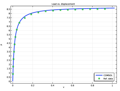
Browse to the model’s Application Libraries folder and double-click the file space_frame_instability_data.txt.

5

In the text field, type Ref data.

1

In the window, right-click and choose .

2

In the window for , locate the section.

3

Find the subsection. From the list, choose .

4

Find the subsection. From the list, choose .

5

In the text field, type 20.

6

Click to expand the section. Select the check box.

7

From the list, choose .

8

In the table, enter the following settings:


Legends
Ref. data

Load vs. displacement

1

In the window, click .

2

In the window for , locate the section.

3

From the list, choose .

4

In the toolbar, click

.

5

button in the toolbar.

Next, you verify the critical buckling load by performing the analysis.

1

In the toolbar, click

to open the window.

2

Go to the window.

3

Find the subsection. In the tree, select .

4

Click in the window toolbar.

5

In the toolbar, click

to close the window.

In the toolbar, click

.

First default plot from the buckling analysis shows the first buckling mode shape as shown in Figure 4.

Mode Shape (beam)

1

In the toolbar, click

.

2

button in the toolbar.