Contact Analysis of an Elastic Snap Hook

PDF

Contact Analysis of an Elastic Snap Hook

In this example, the insertion of a snap hook in to a slot is modeled. The objective is to compute the force needed to place the hook in the slot. The problem thus involves modeling the contact between the hook and the lock during this process.

Model Definition

The geometry of the model is shown in Figure 1. Due to the symmetry, you can study a half of the original snap hook geometry.

Figure 1: Geometry of the modeled half of the snap hook and locking mechanism.

Material Properties

The hook and lock are made of a modified nylon material. However, the hook is assumed rigid in this example. For the hook, a linear elastic material model is used, with material parameters given in the following table:


Material parameter	Value
Young’s modulus	10 GPa
Poisson’s ratio	0.35
Density	1150 kg/m3

Boundary Conditions

•

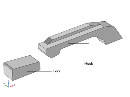
The locking mechanism is considered as rigid, and is modeled as a meshed surface without physics.

•

A prescribed displacement boundary condition is applied at the rightmost bottom surface of the hook. The displacement in the x direction is gradually changed by using the parametric solver; the other two displacement components are zero.

•

Two side boundaries within the xz-plane use symmetry boundary conditions.

•

All the other boundaries are free boundaries. However, several of them are selected as parts of a contact pair with the destination side being on the hook surface.

•

A contact pair is defined with boundaries on the lock selected as source, and boundaries on the hook selected as destination.

•

Contact without friction is considered using the penalty method.

•

Since no physics is defined on the look, it is in the node considered as external to the current physics.

•

The mesh on the source only needs to resolve the geometry of the contact surface. Hence no mesh is needed for the domain, and a refined mesh of the contact surface is only required for the rounded corners of the lock.

Figure 2 shows that the maximum penetration is less than 8 microns during the entire analysis. This is a good accuracy when compared to the geometry size.

Figure 2: Evolution of the maximum penetration for all position of the hook.

Note that the penetration is not constant since the contact force varies depending on the position of the hook.

The maximum equivalent stress levels are found when the displacement of the hook is 3.8 mm, which is just before the hook enters the slot, see Figure 3.

Figure 3: The equivalent stress levels in the hook just before it enters the slot.

Figure 4 shows the force required for the insertion of the hook versus its prescribed displacement. The hook is in its slot at the end of the simulation.

Figure 4: The mounting force as a function of the hook displacement.

Structural_Mechanics_Module/Contact_and_Friction/snap_hook_elastic

Modeling Instructions

From the menu, choose .

In the window, click

.

1

In the window, click

.

2

In the tree, select .

3

4

5

In the tree, select .

6

Global Definitions

1

In the window, under click .

2

In the window for , locate the section.

3

In the table, enter the following settings:


Name	Expression	Value	Description
Displ_max	4.6[mm]	0.0046 m	Maximum hook displacement
disp	0[m]	0 m	Prescribed hook displacement

Import 1 (imp1)

1

In the toolbar, click

.

2

In the window for , locate the section.

3

4

Browse to the model’s Application Libraries folder and double-click the file snap_hook_elastic.mphbin.

5

Rotate 1 (rot1)

1

In the toolbar, click

and choose .

2

Select the object only.

3

In the window for , locate the section.

4

In the text field, type 90.

5

From the list, choose .

6

In the text field, type 1.

7

In the text field, type 0.

8

.

9

button in the toolbar.

1

In the toolbar, click

.

2

In the window for , type contact_src in the text field.

3

Locate the section. From the list, choose .

4

Select the check box.

5

Select Boundaries 1, 4, and 6–8 only.

1

In the toolbar, click

.

2

In the window for , type contact_dst in the text field.

3

Locate the section. From the list, choose .

4

Select Boundaries 14, 15, 20, 22, and 23 only.

Contact Pair 1 (p1)

1

In the toolbar, click

and choose .

2

In the window for , locate the section.

3

From the list, choose .

4

Locate the section. Select the

toggle button.

5

From the list, choose .

Material 1 (mat1)

1

In the window, under right-click and choose .

2

In the window for , locate the section.

3

In the table, enter the following settings:


Property	Variable	Value	Unit	Property group
Young’s modulus	E	10[GPa]	Pa	Basic
Poisson’s ratio	nu	0.35	1	Basic
Density	rho	1150[kg/m^3]	kg/m³	Basic

Solid Mechanics (solid)

1

In the window, under click .

2

In the window for , locate the section.

3

From the list, choose .

4

Select Domains 2 and 3 only.

Prescribed Displacement 1

1

In the toolbar, click

and choose .

2

Select Boundary 30 only.

3

In the window for , locate the section.

4

Select the check box.

5

Select the check box.

6

Select the check box.

7

In the u 0 x text field, type -disp.

1

In the toolbar, click

and choose .

2

Select Boundaries 13 and 19 only.

1

In the toolbar, click

and choose .

2

In the window for , locate the section.

3

Select the check box.

4

Locate the section. Under , click

.

5

In the dialog box, select in the list.

6

7

In the window for , locate the section.

8

From the list, choose .

9

In the fp text field, type 1/10.

Add a structured mesh on the contact destination boundaries.

1

In the toolbar, click

and choose .

2

In the window for , locate the section.

3

From the list, choose .

1

Right-click and choose .

2

Select Edges 27, 28, 39, and 48 only.

3

In the window for , locate the section.

4

In the text field, type 10.

1

In the window, right-click and choose .

2

Select Edges 31 and 45 only.

3

In the window for , locate the section.

4

In the text field, type 4.

5

.

Convert the quad mesh to triangles so that the rest of the geometry can be meshed using the free tetrahedral method.

1

In the toolbar, click

and choose .

2

In the window for , locate the section.

3

From the list, choose .

4

From the list, choose .

5

.

Free Tetrahedral 1

1

In the toolbar, click

.

2

In the window for , locate the section.

3

From the list, choose .

4

Select Domains 2 and 3 only.

1

Right-click and choose .

2

In the window for , locate the section.

3

Click the button.

4

Locate the section. Select the check box.

5

In the associated text field, type 4e-4.

1

In the window, right-click and choose .

Refine the mesh on boundary where high stresses are expected.

2

In the window for , locate the section.

3

From the list, choose .

4

Select Boundary 25 only.

5

Locate the section. Click the button.

6

Locate the section. Select the check box.

7

In the associated text field, type 1e-4.

8

.

Add a surface mesh for the lock. Notice that no mesh is needed for the domain.

1

In the toolbar, click

and choose .

2

In the window for , locate the section.

3

From the list, choose .

1

Right-click and choose .

2

In the window for , locate the section.

3

From the list, choose .

1

In the window, right-click and choose .

2

Select Edges 5 and 13 only.

3

In the window for , locate the section.

4

In the text field, type 10.

5

.

Before setting the study, add a nonlocal integration coupling that will be used for postprocessing the reaction force.

Integration 1 (intop1)

1

In the toolbar, click

and choose .

2

In the window for , locate the section.

3

From the list, choose .

4

Select Boundary 30 only.

5

Locate the section. From the list, choose .

Step 1: Stationary

Set up an auxiliary continuation sweep for the disp parameter.

1

In the window, under click .

2

In the window for , click to expand the section.

3

Select the check box.

4

5

In the table, enter the following settings:


Parameter name	Parameter value list	Parameter unit
disp (Prescribed hook displacement)	range(0.2,1e-2,1)*Displ_max	m

6

Click to expand the section. Select the check box.

7

In the toolbar, click

.

1

In the window for , locate the section.

2

From the list, choose .

3

Locate the section. From the list, choose .

1

In the window, expand the node, then click .

2

In the window for , locate the section.

3

From the list, choose .

Add surface plot of the lock. You can write an arbitrary value in the expression field since a uniform color is used.

1

In the window, right-click and choose .

2

In the window for , locate the section.

3

In the text field, type 1.

4

Click to expand the section. From the list, choose .

5

Click to collapse the section. Locate the section. From the list, choose .

6

From the list, choose .

1

Right-click and choose .

2

In the window for , locate the section.

3

From the list, choose .

4

In the toolbar, click

.

5

button in the toolbar.

Contact Forces (solid)

1

In the window, click .

2

In the window for , locate the section.

3

From the list, choose .

Minimum Gap Distance

1

In the toolbar, click

and choose .

2

In the window for , type Minimum Gap Distance in the text field.

3

Locate the section. Clear the check box.

1

In the toolbar, click

.

2

In the window for , locate the section.

3

In the table, enter the following settings:


Expression	Unit	Description
solid.gapmin_p1*(solid.gapmin_p1<0)	um	Minimum Gap Distance

4

In the toolbar, click

.

1

In the toolbar, click

and choose .

2

In the window for , type Reaction Force in the text field.

3

Locate the section. Clear the check box.

1

In the toolbar, click

.

2

In the window for , locate the section.

3

In the table, enter the following settings:


Expression	Unit	Description
-2*intop1(solid.RFx)	N	Total Force

4

In the toolbar, click

.