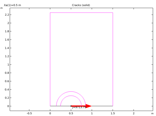
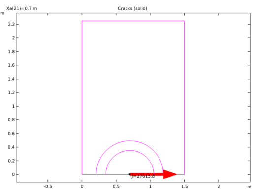
PDF

Single Edge Crack
Introduction
This example deals with the stability of a plate with an edge crack that is subjected to a tensile load. To analyze the stability of existing cracks, you can apply the principles of fracture mechanics.
A common parameter in fracture mechanics, the so-called stress intensity factor KI, provides a means to predict if a specific crack causes the plate to fracture. When this calculated value becomes equal to the critical fracture toughness of the material, KIc (a material property), then usually catastrophic fracture occurs.
Determining the stress intensity factor directly from the local state at the crack tip is problematic, since the stresses are singular there. Because of this, more indirect energy based methods are attractive. In this example, KI is computed using the J-integral and from the energy release rate.
In addition, the crack growth rate and number of cycles needed to propagate the crack a certain distance are computed.
Model Definition
A plate with a width w = 1.5 m and height h = 4.5 m has a single horizontal edge-crack at the middle of the left vertical edge. The length of the crack is varied from a = 0.5 m to a = 0.7 m, see Figure 1. An external load is pulling the plate such that the top and bottom edges experience tensile stress, σ, of 20 MPa.
Because of the symmetry, only half of the plate is modeled. There are three paths for computing the J-integral:
1
2
3
Figure 1: Plate geometry and loading (before applying symmetry conditions).
You apply a tensile load to the upper horizontal edge, while the lower horizontal edge is constrained in the y direction using a symmetry condition. One point is constrained in the horizontal direction in order to suppress rigid body motion.
Material Model
The material properties are representative for steel.
ν
1.4·10-11 (KI unit system: MN/m3/2)
The J-Integral
In this model, you determine the stress intensity factor KI using the so-called J-integral.
The J-integral is a two-dimensional path independent line integral along a counterclockwise contour, Γ, surrounding the crack tip. For a crack extending along the positive x-axis, the J-integral is defined as
where W is the strain energy density
and T is the traction vector defined as
σij denotes the stress components, εij the strain components, and ni the normal vector components.
The J-integral has the following relation to the Mode I stress intensity factor for a plane stress case and a linear elastic material:
(1)
where E is Young’s modulus.
Energy Release Rate
For a linear elastic material it is actually possible to compute the value of the J-integral without using the path integrals. The reason is that its value equals the value of the energy release rate, G,
(2)
Here U is the potential energy, a is the crack length, and t is the thickness. By computing the potential energy for two slightly different crack lengths, G can be estimated as
(3)
The potential energy of an elastic body is
The first term is the strain energy in the volume, and the second term is the potential of the prescribed tractions on the boundary. Because of the linearity,
Thus, it is possible to compute the potential energy using either of these terms independently.
The total strain energy density exists as a built-in variable, making the first expression attractive for determining G.
Crack Propagation
When subjected to a periodic load, the crack growth rate (in meters per load cycle) can be expressed by Paris’ law:
(4)
Here A and m are material parameters and ΔKI is the range of the stress intensity factor. It is assumed that the load varies between 0 and 20 MPa, so that ΔKI equals the computed KI. Note that the value of the coefficient A depends on the unit for the stress intensity factor in a rather complex way because of the power m, which in general is non-integer.
Results
Figure 2 shows the stress singularity at the crack tip.
Figure 2: von Mises stress and the deformed shape of the plate when the crack length is 0.6 m. The displacement is exaggerated to illustrate the deformation under the applied load.
 
Based on Ref. 1 an analytical solution for the stress intensity factor is
where σ = 20 MPa, and f is a correction factor given in Ref. 1.
(5)
The expression in Equation 5 assumes that the plate is long, so that the height is significantly larger than the width. The stress field in Figure 2 indicates that this assumption is fulfilled.
The calculated stress intensity factors for the three different contours, tabulated in the evaluation group Cracks (solid), show excellent agreement with the reference value. The largest deviation for any of the studied crack lengths and integration paths is less than 0.3%.
When using the built-in J-integral computation, you should ascertain that none of the contours used for the integration passes outside the computational domain, or encloses another crack. In the default plot Cracks, all integration paths are visualized. In Figure 3 and Figure 4 the contours are shown for the shortest and longest cracks, respectively.
Figure 3: The contours used for integration when a = 0.5 m.
Figure 4: The contours used for integration when a = 0.7 m.
 
The three different ways of computing the energy release rate, and thus KI, are compared in Figure 5. As can be seen, all three methods give essentially the same values.
Figure 5: J-integral compared with energy release rates computed using numerical differentiation.
Finally, the crack growth speed can be investigated. In Figure 6, the crack growth speed is shown as function of the crack length. The dependence is quite strong: an increase in crack length from 0.5 m to 0.7 m (40%) increases the crack growth rate by a factor of 5. According to the constants used in Paris’ law, the crack growth rate is proportional to the stress intensity factor raised to the power of 3.1. As can be seen from the previous results, the stress intensity factor increases strongly with the crack length, and this combination results in the increase in crack growth rate.
In practice, Paris’ law may not be applicable when KI approaches the critical value KIc.
Figure 6: Crack propagation rate as function of the crack length.
Notes about the COMSOL Implementation
In this analysis you compute the J-integral for three different contours traversing three different regions around the crack tip. Note that the boundaries along the crack are not included in the J-integral because they do not give any contribution to the J-integral. This is due to the following facts: for an ideal crack, dy is zero along the crack faces, and all traction components are also zero (Ti = 0) as the crack faces are not loaded.
To evaluate the J-integral along three different paths, you need to add one Crack node with three J-integral subnodes. Since the Symmetric option is used in the Crack node, the values of the J-integrals and stress intensity factors automatically take the full structure into account.
When you add a J-integral node, the KI, KII, and (in 3D) KIII stress intensity factors are also computed.
When computing the energy release rates, the derivative of the potential energy is computed using a difference approximation. In order to access different solutions in a single expression, the withsol() operator is used.
Reference
1. H Tada, P.C. Paris, and G.R. Irwin, The Stress Analysis of Cracks Handbook, Del Research Corp, Press, 1973.
Application Library path: Structural_Mechanics_Module/Fracture_Mechanics/single_edge_crack
Modeling Instructions
From the File menu, choose New.
New
In the New window, click  Model Wizard.
Model Wizard
1
In the Model Wizard window, click  2D.
2
In the Select Physics tree, select Structural Mechanics>Solid Mechanics (solid).
3
Click Add.
4
Click  Study.
5
In the Select Study tree, select General Studies>Stationary.
6
Global Definitions
Parameters 1
1
In the Model Builder window, under Global Definitions click Parameters 1.
2
In the Settings window for Parameters, locate the Parameters section.
3
Click  Load from File.
4
Geometry 1
Rectangle 1 (r1)
1
In the Geometry toolbar, click  Rectangle.
2
In the Settings window for Rectangle, locate the Size and Shape section.
3
In the Width text field, type Wp.
4
In the Height text field, type Hp.
5
Click  Build All Objects.
Add a point at the crack tip.
Point 1 (pt1)
1
In the Geometry toolbar, click  Point.
2
In the Settings window for Point, locate the Point section.
3
In the x text field, type Xa.
Form Union (fin)
1
In the Model Builder window, click Form Union (fin).
2
In the Settings window for Form Union/Assembly, click  Build Selected.
Materials
Steel
1
In the Model Builder window, under Component 1 (comp1) right-click Materials and choose Blank Material.
2
In the Settings window for Material, type Steel in the Label text field.
3
Locate the Material Contents section. In the table, enter the following settings:
Solid Mechanics (solid)
1
In the Model Builder window, under Component 1 (comp1) click Solid Mechanics (solid).
2
In the Settings window for Solid Mechanics, locate the 2D Approximation section.
3
4
Locate the Thickness section. In the d text field, type Th.
Symmetry 1
1
In the Physics toolbar, click  Boundaries and choose Symmetry.
2
It does not matter whether you select boundary 2 as a symmetry boundary or not. If selected, it will be overridden when the Crack node is added.
Boundary Load 1
1
In the Physics toolbar, click  Boundaries and choose Boundary Load.
2
3
In the Settings window for Boundary Load, locate the Force section.
4
Specify the FA vector as
Prescribed Displacement 1
1
In the Physics toolbar, click  Points and choose Prescribed Displacement.
Suppress rigid body motion.
2
3
In the Settings window for Prescribed Displacement, locate the Prescribed Displacement section.
4
Select the Prescribed in x direction check box.
Crack 1
1
In the Physics toolbar, click  Boundaries and choose Crack.
2
In the Settings window for Crack, locate the Crack Definition section.
3
From the Crack surface list, choose Symmetric.
4
5
Click to expand the Crack Front section. Click  Clear Selection.
6
J-Integral 1
In the Physics toolbar, click  Attributes and choose J-Integral.
J-Integral 2
1
Right-click J-Integral 1 and choose Duplicate.
2
In the Settings window for J-Integral, locate the J-Integral section.
3
In the rΓ text field, type solid.crack1.crackSize*0.7.
Crack 1
In the Model Builder window, click Crack 1.
J-Integral 3
1
In the Physics toolbar, click  Attributes and choose J-Integral.
2
In the Settings window for J-Integral, locate the J-Integral section.
3
From the Integration path list, choose On edges.
4
5
Locate the Integration Path section. Select the  Activate Selection toggle button.
6
Definitions
Loaded edge integration
1
In the Definitions toolbar, click  Nonlocal Couplings and choose Integration.
2
In the Settings window for Integration, type Loaded edge integration in the Label text field.
3
In the Operator name text field, type LoadEdgeInt.
4
Locate the Source Selection section. From the Geometric entity level list, choose Boundary.
5
Use a fine mesh close to the crack tip where the stress gradients are large. The Crack node will automatically provide that, but you may want to adjust the settings manually.
Mesh 1
1
In the Model Builder window, under Component 1 (comp1) click Mesh 1.
2
In the Settings window for Mesh, locate the Physics-Controlled Mesh section.
3
From the Element size list, choose Finer.
4
Locate the Mesh Settings section. From the Sequence type list, choose User-controlled mesh.
Size 1
1
In the Model Builder window, under Component 1 (comp1)>Mesh 1 click Size 1.
2
In the Settings window for Size, locate the Element Size section.
3
Click the Custom button.
4
Locate the Element Size Parameters section. Select the Maximum element size check box.
5
6
Click  Build All.
Set up a parametric sweep over the crack length.
Study 1
Parametric Sweep
1
In the Study toolbar, click  Parametric Sweep.
2
In the Settings window for Parametric Sweep, locate the Study Settings section.
3
4
5
In the Study toolbar, click  Compute.
Results
Mirror 2D 1
1
In the Results toolbar, click  More Datasets and choose Mirror 2D.
2
In the Settings window for Mirror 2D, locate the Axis Data section.
3
In row Point 2, set X to 1.
4
In row Point 2, set Y to 0.
5
Locate the Data section. From the Dataset list, choose Study 1/Parametric Solutions 1 (sol2).
Stress (solid)
1
In the Model Builder window, click Stress (solid).
2
In the Settings window for 2D Plot Group, locate the Data section.
3
From the Dataset list, choose Mirror 2D 1.
4
From the Parameter value (Xa (m)) list, choose 0.6.
5
Locate the Plot Settings section. Clear the Plot dataset edges check box.
Surface 1
1
In the Model Builder window, expand the Stress (solid) node, then click Surface 1.
2
In the Settings window for Surface, locate the Expression section.
3
From the Unit list, choose MPa.
4
Click to expand the Range section. Select the Manual color range check box.
5
In the Minimum text field, type 0.
6
In the Maximum text field, type 100.
7
Click to expand the Quality section. From the Smoothing list, choose None.
Applied Loads (solid)
In the Model Builder window, expand the Results>Applied Loads (solid) node.
Boundary Load 1
1
In the Model Builder window, expand the Results>Applied Loads (solid)>Boundary Loads (solid) node.
2
Right-click Boundary Load 1 and choose Copy.
Boundary Load 1
1
In the Model Builder window, right-click Stress (solid) and choose Paste Arrow Line.
2
In the Settings window for Arrow Line, click to expand the Inherit Style section.
3
From the Plot list, choose Surface 1.
4
Clear the Arrow scale factor check box.
5
Clear the Color check box.
6
Clear the Color and data range check box.
7
Click to expand the Title section. From the Title type list, choose None.
8
Locate the Coloring and Style section. Select the Scale factor check box.
9
Color Expression
1
In the Model Builder window, expand the Boundary Load 1 node, then click Color Expression.
2
In the Settings window for Color Expression, locate the Coloring and Style section.
3
Clear the Color legend check box.
Deformation
1
In the Model Builder window, expand the Results>Stress (solid)>Surface 1 node, then click Deformation.
2
In the Settings window for Deformation, locate the Scale section.
3
Select the Scale factor check box.
4
5
In the Stress (solid) toolbar, click  Plot.
6
Click the  Zoom Extents button in the Graphics toolbar.
Check the placement of the integration contours. In particular, it must be ensured that the circular paths are inside the domain.
Cracks (solid)
1
In the Model Builder window, click Cracks (solid).
2
In the Cracks (solid) toolbar, click  Plot.
3
In the Settings window for 2D Plot Group, click  Plot First.
Check if there are any differences between the results for the three contours. That could indicate a too coarse mesh.
Since this is a pure Mode I case, remove the evaluation of the Mode II stress intensity factors.
Stress Intensity Factors, Mode II
1
In the Model Builder window, expand the Cracks (solid) node.
2
Right-click Stress Intensity Factors, Mode II and choose Delete.
Stress Intensity Factors, Mode I
Add a comparison between the values from the second integration path and the reference stress intensity factor.
1
In the Model Builder window, click Stress Intensity Factors, Mode I.
2
In the Settings window for Global Evaluation, locate the Expressions section.
3
4
In the Cracks (solid) toolbar, click  Evaluate.
Table
1
Go to the Table window.
Compare the J-integral with an energy release rate based on numerical differentiation of the strain energy with respect to the crack length.
Definitions
Variables 1
1
In the Model Builder window, under Component 1 (comp1) right-click Definitions and choose Variables.
2
In the Settings window for Variables, locate the Variables section.
3
After having added a new variable, you must update the solution to make it accessible for result presentation.
Study 1
In the Study toolbar, click  Update Solution.
Results
J-integral and G
1
In the Home toolbar, click  Add Plot Group and choose 1D Plot Group.
2
In the Settings window for 1D Plot Group, type J-integral and G in the Label text field.
3
Locate the Data section. From the Dataset list, choose Study 1/Parametric Solutions 1 (sol2).
4
From the Parameter selection (Xa) list, choose Manual.
5
In the Parameter indices (1-21) text field, type range(2,20).
Global 1
1
Right-click J-integral and G and choose Global.
2
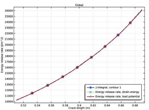
In the Settings window for Global, click Replace Expression in the upper-right corner of the y-Axis Data section. From the menu, choose Component 1 (comp1)>Solid Mechanics>Cracks>solid.crack1.jint1.J - J-integral - J/m².
3
Locate the y-Axis Data section. In the table, enter the following settings:
4
Click to expand the Coloring and Style section. Find the Line style subsection. From the Line list, choose Cycle.
5
In the Width text field, type 2.
6
Find the Line markers subsection. From the Marker list, choose Cycle.
J-integral and G
1
In the Model Builder window, click J-integral and G.
2
In the Settings window for 1D Plot Group, locate the Plot Settings section.
3
Select the x-axis label check box.
4
5
Select the y-axis label check box.
6
In the associated text field, type Energy release rate (J/m^2).
7
Locate the Legend section. From the Position list, choose Lower right.
8
In the J-integral and G toolbar, click  Plot.
Crack growth rate
1
In the Home toolbar, click  Add Plot Group and choose 1D Plot Group.
2
In the Settings window for 1D Plot Group, type Crack growth rate in the Label text field.
3
Locate the Data section. From the Dataset list, choose Study 1/Parametric Solutions 1 (sol2).
Global 1
1
Right-click Crack growth rate and choose Global.
2
In the Settings window for Global, locate the y-Axis Data section.
3
4
Locate the Coloring and Style section. In the Width text field, type 2.
Crack growth rate
1
In the Model Builder window, click Crack growth rate.
2
In the Settings window for 1D Plot Group, click to expand the Title section.
3
From the Title type list, choose None.
4
Locate the Plot Settings section. Select the x-axis label check box.
5
6
Select the y-axis label check box.
7
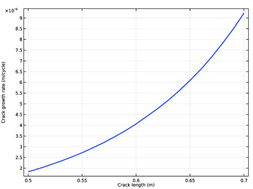
In the associated text field, type Crack growth rate (m/cycle).
8
Locate the Legend section. Clear the Show legends check box.
9
In the Crack growth rate toolbar, click  Plot.
Compute the total number of cycles needed for driving the crack from 0.5 m to 0.7 m.
Number of cycles
1
In the Results toolbar, click  Global Evaluation.
2
In the Settings window for Global Evaluation, type Number of cycles in the Label text field.
3
Locate the Data section. From the Dataset list, choose Study 1/Parametric Solutions 1 (sol2).
4
Locate the Expressions section. In the table, enter the following settings:
5
Locate the Data Series Operation section. From the Operation list, choose Integral.
6
Click  Evaluate.