Modeling Rigid Bodies

In many structural dynamics applications, some components are stiff compared to the supporting structure. Such a stiff part only contributes to the dynamic properties of the structure through its mass and moment of inertia. It is then possible to reduce the model size significantly by treating it as a rigid body.

In this example you compute the eigenfrequency of an assembly where one of the parts can be considered as a rigid domain.

Model Definition

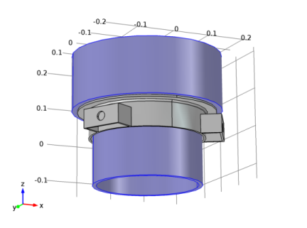
An aluminum frame supports a heavy solid part made of steel. Due to the difference in stiffness between the two domains, the steel component can be regarded as rigid.

Figure 1 below shows the assembly geometry with the aluminum bracket shown in gray and the steel domain shown in blue.

Figure 1: Model geometry with the rigid steel domain shown in blue.

The mounting frame is fixed at the three bolt holes and an eigenfrequency analysis is performed to find the first six natural frequencies of the assembly.

Results and Discussion

The plots in Figure 2 below show the eigenmodes for the first six natural frequencies.

Figure 2: Displacement field for the six lowest eigenmodes.

Eigenfrequencies which are close to each other indicates that corresponding eigenmodes can be similar but due to the model symmetry they occur in different directions. Compare modes 1 with 2 and 5 with 6 in Figure 2.

Notes About the COMSOL Implementation

In COMSOL Multiphysics you can define a rigid domain as a special material model. The mass and moment of inertia properties are then computed, and the rigid domain is represented by only seven degrees of freedom: three for the translations and four for the rotations. The four rotational degrees of freedom are quaternion components which together represent a rotation vector and the rotation angle.

The rigid part still needs to have a mesh, because a numerical integration is performed over the domain in order to obtain the mass properties.The mesh can however be very coarse.

Structural_Mechanics_Module/Connectors_and_Mechanisms/rigid_domain

Modeling Instructions

From the menu, choose .

New

In the window, click

Model Wizard

In the window, click

In the tree, select .

Click .

Click

In the tree, select .

Click

Geometry 1

Import 1 (imp1)

In the toolbar, click

In the window for , locate the section.

Click .

Browse to the model’s Application Libraries folder and double-click the file rigid_domain.mphbin.

Click .

Form Union (fin)

In the window, click .

In the window for , click

Add Material

In the toolbar, click

to open the window.

Go to the window.

In the tree, select .

Click in the window toolbar.

In the tree, select .

Click in the window toolbar.

In the toolbar, click

to close the window.

Materials

Structural steel (mat2)

Select Domain 2 only.

Solid Mechanics (solid)

Fixed Constraint 1

In the window, under right-click and choose .

Select Boundaries 11, 12, 28, 29, 48, and 49 only.

Rigid Domain 1

In the toolbar, click

and choose .

Select Domain 2 only.

Study 1

In the toolbar, click

Results

Mode Shape (solid)

The default plot shows the mode shape for the first resonance frequency. To improve the visualization, add an arrow plot of the displacements.

Arrow Surface 1

Right-click and choose .

Deformation 1

In the window, right-click and choose .

Arrow Surface 1

In the window for , click to expand the section.

From the list, choose .

Click to expand the section. From the list, choose .

Locate the section. In the text field, type 100.

Locate the section. Select the check box.

In the associated text field, type 2e5.

Surface 1

In the window, click .

In the window for , click to expand the section.

From the list, choose .

To view the solution for the other eigenfrequencies shown in Figure 2, do the following:

In the settings window, click the button to display the solution from the next eigenfrequency.