PDF

Failure Prediction in a Layered Shell
Introduction
Laminated shells made of carbon fiber reinforced plastic (CRFP) are common in a large variety of applications due to their high strength to weight ratio. Evaluation of the structural integrity of a laminated shell for a set of applied loads is necessary to make the design of such structures reliable.
This example shows how to model laminated shells using an ordinary Linear Elastic Material model in the Shell interfaces available with the Structural Mechanics Module. The same example can be modeled using a Layered Linear Elastic Material model in the Shell interface. The model using the latter approach can be found in the Verification Examples folder of the Composite Materials Application Library.
The structural integrity of a stack of shells with different fiber orientations is assessed through the parameters called Failure Index and Safety Factor, using different polynomial failure criteria. Because of the orientation, each ply will have different strength in the longitudinal and transversal direction, and hence different response to the loading. The analysis using a polynomial failure criterion is termed first ply failure analysis, where failure in any ply is considered as failure of the whole laminate. In this example, seven different polynomial criteria are compared.
The original model is a NAFEMS benchmark model, described in Benchmarks for Membrane and Bending Analysis of Laminated Shells, Part 2: Strength Analysis (Ref. 1). The COMSOL Multiphysics solutions are compared with the reference data.
Model Definition
The physical geometry of the problem consists of four square shells stacked above each other. The side length is 1 cm and each layer has thickness of 0.05 mm. The laminate (90/-45/45/0) is subjected to an in-plane axial tensile load. The actual geometry of the laminate is shown in Figure 1.
Figure 1: Geometry of layered shell with ply orientations 90/-45/45/0 from top to bottom.
Material Properties
The orthotropic material properties (Young’s modulus, shear modulus, and Poisson’s ratio) are given in Table 1:
{E1,E2,E3}
{G12,G23,G13}
{υ12,υ23,υ13}
The tensile, compressive, and shear strengths are given in Table 2.
{σt1,σt2,σt3}
{σc1,σc2,σc3}
{σss23,σss13,σss12}
All material properties and strengths are given in the local material directions, where the first axis is aligned with the fiber orientation.
Boundary Conditions
The applied boundary conditions and loads on each node are given in the table below.
u, v, w, θx, θy, θz
θz
θz
u, θz
The numbers within parenthesis are point numbers in COMSOL Multiphysics geometry. The boundary conditions provided in the benchmark specifications apply to the layered shell as a single entity. The rotation around the z-axis, θz, is automatically constrained so it does not need to be considered.
Failure Criteria
Seven different failure criteria are used to predict the failure in the layered shell. These are Tsai–Wu anisotropic, Tsai–Wu orthotropic, Tsai–Hill, Hoffman, Modified Tsai–Hill, Azzi–Tsai–Hill, and Norris criteria.
Tsai–Wu Anisotropic
For the Tsai–Wu anisotropic criterion, the material strength parameters are taken from Table 2 in order to obtain the same results as with the Tsai–Wu orthotropic criterion. This exercise is done in order to verify the correctness of the implementation. The nonzero elements in the second rank tensor f are given below. Here, and in the following equations, repeated indices do not imply summation.
(1)
The nonzero elements in the fourth rank tensor F are
(2)
Modified Tsai–Hill Orthotropic
The Hill criterion in Ref. 1 is called the Modified Tsai–Hill criterion in COMSOL Multiphysics.
Ref. 1 does not give results for the Tsai–Wu anisotropic, Tsai–Hill, Azzi–Tsai–Hill, and Norris criteria; so the analytical results for failure index and safety factor are here derived from the stress values given in Ref. 1.
The stresses from Ref. 1 are given in Table 4. Apart from σ11, σ22, and σ12, all other stress components are either zero or negligible.
σ11 (MPa)
σ22 (MPa)
σ12 (MPa)
For all the selected polynomial criteria, the failure index (FI) is written as
(3)
where σi is the 6-by-1 stress vector (sorted using Voigt notation), Fij is a 6-by-6 symmetric matrix (fourth rank tensor) that contains the coefficients for the quadratic terms, and fi is a 6-by-1 vector (second rank tensor) that contains the linear terms. A failure index equal to or greater than 1.0 indicates failure in the material. In order to find the safety factor SF, the applied stress in Equation 3 is multiplied by the safety factor SF, and the failure index FI is set equal to 1.0, which results in a quadratic equation of the form
(4)
where and .
The lowest positive root in Equation 4 is selected as the safety factor. Based on the stress values given in Table 4, the failure index and safety factor are computed for the criteria for which results in Ref. 1 are missing.
Tsai–Wu Anisotropic
For the Tsai–Wu anisotropic criterion, the nonzero elements of the vector fi and the matrix Fij are given by Equation 1 and Equation 2. By taking values of stresses from Table 4, the failure index and safety factor are computed from Equation 3 and Equation 4, and given in Table 5 below.
FI
SF
Tsai–Hill Orthotropic
For the Tsai–Hill orthotropic criterion, all elements of the vector fi are zero, while the nonzero elements of the matrix Fij are given by the Equation 5.
(5)
By taking values of stresses from Table 4, the failure index and safety factor are computed from Equation 3, Equation 4, and Equation 5, and given in Table 6 below.
FI
SF
Azzi–Tsai–Hill
For the Azzi–Tsai–Hill criterion, all elements of the vector fi are zero, while the nonzero elements of the matrix Fij are given by Equation 6.
(6)
By taking values of the stresses from Table 4, the failure index and safety factor are computed from Equation 3, Equation 4, and Equation 6, and given in Table 7 below.
FI
SF
Norris
For the Norris criterion, all elements of the vector fi are zero, while the nonzero elements of the matrix Fij are given by Equation 7.
(7)
By taking values of the stresses from Table 4, the failure index and safety factor are computed from Equation 3, Equation 4, and Equation 7, and given in Table 8 below.
FI
SF
Note that for the current model, failure index and safety factor are computed at the midplane of each shell interface. However, COMSOL Multiphysics actually computes failure index, safety factor, damage index, and margin of safety at bottom, middle, and top surfaces of the shell, as well as the most critical of the three values.
Results and Discussion
The computed stresses are shown in Table 4, while Table 5 through Table 8 show the analytical values for failure index and safety factor (reserve factor) for certain failure criteria. For the Tsai–Wu orthotropic, Modified Tsai–Hill, and Hoffman criteria, the failure index and safety factor are taken from Ref. 1. The results are compared with results from COMSOL Multiphysics.
σ11 from benchmark
σ11, computed
σ22 from benchmark
σ22, computed
σ12 from benchmark
σ12, computed
 
 
For many industrial and real life applications, the safety factor (SF) is more useful than the failure index (FI). The safety factor (or reserve factor) gives a direct indication of how close the component is to failure. Figure 2 shows the Hoffman safety factor (SF) at the midplane for the different plies. Ply 1 (90-degree ply) is close to failure as expected because of its orientation, where fibers are perpendicular to the loading direction.
Figure 2: Hoffman safety factors at midplanes for a stack of shells.
The von Mises stresses in all plies are shown in Figure 3. The stress in ply 1 is the lowest, but this layer is still more susceptible to failure due to the orientation of its fibers.
Figure 3: von Mises stress in a stack of shells.
Notes About the COMSOL Implementation
This layered shell is modeled using four separate Shell interfaces on top of each other. All four interfaces are located on the same boundary, and share the translational and rotational degrees of freedom. It is only the different values of the offset properties which describes the stacking.
The boundary conditions provided in the benchmark specifications apply to the layered shell as a single entity. When implemented in this model, special attention must be paid to the boundary condition stating that in one point, only the x-translation should be constrained. In the shell sense, this is a condition on the midsurface of the stack, which is between ply 2 and ply 3. Setting the degree of freedom u to zero, would in this case imply that also the rotation around the y-axis is constrained, since it would be applied on all layers. The intended boundary condition is instead implemented by stating that the x-displacement in ply 3 should be the negative of the x-displacement in ply 2.
Reference
1. P. Hopkins, Benchmarks for Membrane and Bending Analysis of Laminated Shells, Part 2: Strength Analysis, NAFEMS, 2005.
Application Library path: Structural_Mechanics_Module/Verification_Examples/failure_prediction_in_a_layered_shell
Modeling Instructions
From the File menu, choose New.
New
In the New window, click  Model Wizard.
Model Wizard
1
In the Model Wizard window, click  3D.
2
In the Select Physics tree, select Structural Mechanics>Shell (shell).
3
Click Add.
4
In the Select Physics tree, select Structural Mechanics>Shell (shell).
5
Click Add.
6
In the Select Physics tree, select Structural Mechanics>Shell (shell).
7
Click Add.
8
In the Select Physics tree, select Structural Mechanics>Shell (shell).
9
Click Add.
10
Click  Study.
11
In the Select Study tree, select General Studies>Stationary.
12
Global Definitions
Parameters 1
Load the text file containing the material properties and material strengths.
1
In the Model Builder window, under Global Definitions click Parameters 1.
2
In the Settings window for Parameters, locate the Parameters section.
3
Click  Load from File.
4
Browse to the model’s Application Libraries folder and double-click the file failure_prediction_in_a_layered_shell_materialproperties.txt.
Definitions
Set up three rotated coordinate systems.
Rotated System 2 (sys2)
1
In the Definitions toolbar, click  Coordinate Systems and choose Rotated System.
2
In the Settings window for Rotated System, locate the Rotation section.
3
Find the Euler angles (Z-X-Z) subsection. In the α text field, type pi/2.
Rotated System 3 (sys3)
1
Right-click Rotated System 2 (sys2) and choose Duplicate.
2
In the Settings window for Rotated System, locate the Rotation section.
3
Find the Euler angles (Z-X-Z) subsection. In the α text field, type -pi/4.
Rotated System 4 (sys4)
1
Right-click Rotated System 3 (sys3) and choose Duplicate.
2
In the Settings window for Rotated System, locate the Rotation section.
3
Find the Euler angles (Z-X-Z) subsection. In the α text field, type pi/4.
Geometry 1
Work Plane 1 (wp1)
In the Geometry toolbar, click  Work Plane.
Work Plane 1 (wp1)>Plane Geometry
In the Model Builder window, click Plane Geometry.
Work Plane 1 (wp1)>Square 1 (sq1)
1
In the Work Plane toolbar, click  Square.
2
In the Settings window for Square, locate the Size section.
3
In the Side length text field, type 1e-2.
4
Click  Build Selected.
5
Click the  Zoom Extents button in the Graphics toolbar.
Materials
Material 1 (mat1)
In the Model Builder window, under Component 1 (comp1) right-click Materials and choose Blank Material.
Ply 1
Activate Advanced Physics option from Show button.
1
Click the  Show More Options button in the Model Builder toolbar.
2
In the Show More Options dialog box, in the tree, select the check box for the node Physics>Advanced Physics Options.
3
The layered shell is modeled using four separate shell interfaces located on the same boundary (mesh surface), sharing the degrees of freedom. The stacking of the shells is done using a Physical Offset option. With this option the constraints and loads are transferred to the actual midplane of the shells without modeling it.
As the same degrees of freedom are to be shared by all shell interfaces, set the displacement field to u and the displacement of the shell normals to ar for Shell 2, Shell 3, and Shell 4.
Set the discretization for the displacement field to Linear in order to resemble the benchmark example.
The results given in the benchmark example are at the midplane of each shell layer. Set the Default Through-Thickness Result Location to zero for all shells.
4
In the Settings window for Shell, type Ply 1 in the Label text field.
5
In the Name text field, type shell1.
6
Click to expand the Default Through-Thickness Result Location section. In the z text field, type 0.
7
Click to expand the Discretization section. From the Displacement field list, choose Linear.
Thickness and Offset 1
1
In the Model Builder window, under Component 1 (comp1)>Ply 1 (shell1) click Thickness and Offset 1.
2
In the Settings window for Thickness and Offset, locate the Thickness and Offset section.
3
In the d text field, type th.
4
From the Offset definition list, choose Physical offset.
5
In the zoffset text field, type 1.5*th.
Linear Elastic Material 1
Choose the orthotropic solid model for the linear elastic material and assign Rotated System 2 as Shell Local System.
1
In the Model Builder window, click Linear Elastic Material 1.
2
In the Settings window for Linear Elastic Material, locate the Linear Elastic Material section.
3
From the Solid model list, choose Orthotropic.
Shell Local System 1
1
In the Model Builder window, click Shell Local System 1.
2
In the Settings window for Shell Local System, locate the Coordinate System Selection section.
3
From the Coordinate system list, choose Rotated System 2 (sys2).
Ply 2
1
In the Model Builder window, under Component 1 (comp1) click Shell 2 (shell2).
2
In the Settings window for Shell, type Ply 2 in the Label text field.
3
Locate the Discretization section. From the Displacement field list, choose Linear.
4
Locate the Default Through-Thickness Result Location section. In the z text field, type 0.
5
Click to expand the Dependent Variables section. In the Displacement field text field, type u.
6
In the Displacement of shell normals text field, type ar.
Thickness and Offset 1
1
In the Model Builder window, under Component 1 (comp1)>Ply 2 (shell2) click Thickness and Offset 1.
2
In the Settings window for Thickness and Offset, locate the Thickness and Offset section.
3
In the d text field, type th.
4
From the Offset definition list, choose Physical offset.
5
In the zoffset text field, type 0.5*th.
Linear Elastic Material 1
Choose the orthotropic solid model for the linear elastic material and assign Rotated System 3 as Shell Local System.
1
In the Model Builder window, click Linear Elastic Material 1.
2
In the Settings window for Linear Elastic Material, locate the Linear Elastic Material section.
3
From the Solid model list, choose Orthotropic.
Shell Local System 1
1
In the Model Builder window, click Shell Local System 1.
2
In the Settings window for Shell Local System, locate the Coordinate System Selection section.
3
From the Coordinate system list, choose Rotated System 3 (sys3).
Ply 3
1
In the Model Builder window, under Component 1 (comp1) click Shell 3 (shell3).
2
In the Settings window for Shell, type Ply 3 in the Label text field.
3
Locate the Discretization section. From the Displacement field list, choose Linear.
4
Locate the Default Through-Thickness Result Location section. In the z text field, type 0.
5
Locate the Dependent Variables section. In the Displacement field text field, type u.
6
In the Displacement of shell normals text field, type ar.
Thickness and Offset 1
1
In the Model Builder window, under Component 1 (comp1)>Ply 3 (shell3) click Thickness and Offset 1.
2
In the Settings window for Thickness and Offset, locate the Thickness and Offset section.
3
In the d text field, type th.
4
From the Offset definition list, choose Physical offset.
5
In the zoffset text field, type -0.5*th.
Linear Elastic Material 1
Choose the orthotropic solid model for the linear elastic material and assign Rotated System 4 as Shell Local System.
1
In the Model Builder window, click Linear Elastic Material 1.
2
In the Settings window for Linear Elastic Material, locate the Linear Elastic Material section.
3
From the Solid model list, choose Orthotropic.
Shell Local System 1
1
In the Model Builder window, click Shell Local System 1.
2
In the Settings window for Shell Local System, locate the Coordinate System Selection section.
3
From the Coordinate system list, choose Rotated System 4 (sys4).
Ply 4
1
In the Model Builder window, under Component 1 (comp1) click Shell 4 (shell4).
2
In the Settings window for Shell, type Ply 4 in the Label text field.
3
Locate the Discretization section. From the Displacement field list, choose Linear.
4
Locate the Default Through-Thickness Result Location section. In the z text field, type 0.
5
Locate the Dependent Variables section. In the Displacement field text field, type u.
6
In the Displacement of shell normals text field, type ar.
Thickness and Offset 1
1
In the Model Builder window, under Component 1 (comp1)>Ply 4 (shell4) click Thickness and Offset 1.
2
In the Settings window for Thickness and Offset, locate the Thickness and Offset section.
3
In the d text field, type th.
4
From the Offset definition list, choose Physical offset.
5
In the zoffset text field, type -1.5*th.
Linear Elastic Material 1
1
In the Model Builder window, click Linear Elastic Material 1.
2
In the Settings window for Linear Elastic Material, locate the Linear Elastic Material section.
3
From the Solid model list, choose Orthotropic.
Materials
Material 1 (mat1)
Select the material properties for the orthotropic material from Table 1.
1
In the Model Builder window, under Component 1 (comp1)>Materials click Material 1 (mat1).
2
In the Settings window for Material, locate the Material Contents section.
3
Ply 1 (shell1)
Linear Elastic Material 1
In the Model Builder window, under Component 1 (comp1)>Ply 1 (shell1) click Linear Elastic Material 1.
Safety: Tsai-Wu Orthotropic Criterion
1
In the Physics toolbar, click  Attributes and choose Safety.
2
In the Settings window for Safety, type Safety: Tsai-Wu Orthotropic Criterion in the Label text field.
3
Locate the Failure Model section. From the Failure criterion list, choose Tsai-Wu orthotropic.
Safety 2, 3, 4, 5, 6, 7
1
Create six similar Safety nodes by duplicating the Safety 1 node, and replace the failure criterion as given in the table below:
Select all Safety nodes under Play 1 (shell1)>> Linear Elastic Material 1, and right click to Copy. Then, go to Linear Elastic Material 1 under Play 2 (shell2), Play 3 (shell3), and Ply 4 (shell4) and right click to Paste Mutiple Items.
Materials
Material 1 (mat1)
Enter the material properties for the Tsai-Wu Anisotropic criterion as shown in Equation 1 and Equation 2.
1
In the Model Builder window, under Component 1 (comp1)>Materials click Material 1 (mat1).
2
In the Settings window for Material, locate the Material Contents section.
3
Ply 1 (shell1)
Fixed Constraint 1
1
In the Physics toolbar, click  Points and choose Fixed Constraint.
2
Apply a nodal tensile load of 15 N as an edge load. The load is shared by all shell midplanes, hence it is divided by 4 in order to keep a total value of 15 N.
Edge Load 1
1
In the Physics toolbar, click  Edges and choose Edge Load.
2
3
In the Settings window for Edge Load, locate the Force section.
4
From the Load type list, choose Total force.
5
Specify the Ftot vector as
Now select Fixed Constraint and Edge Load nodes under Ply 1 (shell1), and right click to Copy. Then go to Ply 2 (shell2), Ply 3 (shell3), and Ply 4 (shell4); and right click to Paste Mutiple Items.
Ply 2 (shell2)
To enforce a fixed x-direction translation on Node 2, apply the displacement u0 in the x direction to Point 2 of shell2, and the displacement -u0 in the x direction to the same point of shell3. Also add a Global Equation node under shell3 for the additional degree of freedom u0.
1
In the Model Builder window, under Component 1 (comp1) click Ply 2 (shell2).
Prescribed Displacement/Rotation 1
1
In the Physics toolbar, click  Points and choose Prescribed Displacement/Rotation.
2
3
In the Settings window for Prescribed Displacement/Rotation, locate the Prescribed Displacement section.
4
Select the Prescribed in x direction check box.
5
In the u0x text field, type u0.
Ply 3 (shell3)
1
In the Model Builder window, under Component 1 (comp1) click Ply 3 (shell3).
2
In the Physics toolbar, click  Points and choose Prescribed Displacement/Rotation.
Prescribed Displacement/Rotation 1
1
2
In the Settings window for Prescribed Displacement/Rotation, locate the Prescribed Displacement section.
3
Select the Prescribed in x direction check box.
4
In the u0x text field, type -u0.
5
Click the  Show More Options button in the Model Builder toolbar.
6
In the Show More Options dialog box, in the tree, select the check box for the node Physics>Equation-Based Contributions.
7
Global Equations 1
1
In the Physics toolbar, click  Global and choose Global Equations.
2
In the Settings window for Global Equations, locate the Global Equations section.
3
4
Locate the Units section. Click  Select Dependent Variable Quantity.
5
In the Physical Quantity dialog box, type displacement in the text field.
6
Click  Filter.
7
In the tree, select General>Displacement (m).
8
Mesh 1
Use a single quadrilateral element.
Free Quad 1
1
In the Mesh toolbar, click  Boundary and choose Free Quad.
2
Distribution 1
1
Right-click Free Quad 1 and choose Distribution.
2
In the Settings window for Distribution, locate the Edge Selection section.
3
From the Selection list, choose All edges.
4
Locate the Distribution section. In the Number of elements text field, type 1.
5
Click  Build All.
Study 1
Switch off the generation of default plots, since each Shell interface will generate three plots by default.
1
In the Model Builder window, click Study 1.
2
In the Settings window for Study, locate the Study Settings section.
3
Clear the Generate default plots check box.
4
In the Home toolbar, click  Compute.
Results
In the Model Builder window, expand the Results node.
Cut Point 3D 1
1
In the Model Builder window, expand the Results>Datasets node.
2
Right-click Results>Datasets and choose Cut Point 3D.
3
In the Settings window for Cut Point 3D, locate the Point Data section.
4
In the X text field, type 0.5e-2.
5
In the Y text field, type 0.5e-2.
6
In the Z text field, type 0.
Failure indices in Ply 1
1
In the Results toolbar, click  Point Evaluation.
2
In the Settings window for Point Evaluation, type Failure indices in Ply 1 in the Label text field.
3
Locate the Data section. From the Dataset list, choose Cut Point 3D 1.
4
Locate the Expressions section. In the table, enter the following settings:
5
Click  Evaluate.
Failure indices in Ply 1
1
In the Model Builder window, expand the Results>Tables node, then click Table 1.
2
In the Settings window for Table, type Failure indices in Ply 1 in the Label text field.
Point Evaluation 2, 3, 4
Create three similar Point Evaluation nodes by duplicating the Point Evaluation 1 node, and replace the word shell1 in the Expressions by shell2, shell3, and shell4 for Point Evaluation 2, Point Evaluation 3, and Point Evaluation 4, respectively. Rename point evaluation nodes and tables appropriately.
Safety factors in Ply 1
1
In the Results toolbar, click  Point Evaluation.
2
In the Settings window for Point Evaluation, type Safety factors in Ply 1 in the Label text field.
3
Locate the Data section. From the Dataset list, choose Cut Point 3D 1.
4
Locate the Expressions section. In the table, enter the following settings:
5
Click  Evaluate.
Safety factors in Ply 1
1
In the Model Builder window, under Results>Tables click Table 5.
2
In the Settings window for Table, type Safety factors in Ply 1 in the Label text field.
Point Evaluation 6, 7, 8
Create three similar Point Evaluation nodes by duplicating the Point Evaluation 5 node and replace the word shell1 in the Expressions by shell2, shell3, and shell4 for Point Evaluation 6, Point Evaluation 7, and Point Evaluation 8, respectively. Rename them appropriately.
Stresses in Ply 1
1
In the Results toolbar, click  Point Evaluation.
2
In the Settings window for Point Evaluation, type Stresses in Ply 1 in the Label text field.
3
Locate the Data section. From the Dataset list, choose Cut Point 3D 1.
4
Locate the Expressions section. In the table, enter the following settings:
5
Click  Evaluate.
Stresses in Ply 1
1
In the Model Builder window, under Results>Tables click Table 9.
2
In the Settings window for Table, type Stresses in Ply 1 in the Label text field.
Point Evaluation 10, 11, 12
Create three similar Point Evaluation nodes by duplicating the Point Evaluation 9 node, and replace the word shell1 in the Expressions by shell2, shell3, and shell4 for Point Evaluation 10, Point Evaluation 11, and Point Evaluation 12, respectively. Rename them appropriately.
To visualize von Mises stress in the layered shell, use four different Surface plots for four shells in the 3D Plot Group. Modify the Z component in the Deformation node for each surface in order to visualize it better.
von Mises Stress in Stack of Shells
1
In the Results toolbar, click  3D Plot Group.
2
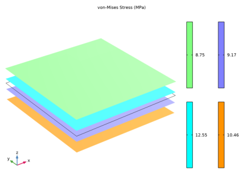
In the Settings window for 3D Plot Group, type von Mises Stress in Stack of Shells in the Label text field.
3
Click to expand the Title section. From the Title type list, choose Manual.
4
In the Title text area, type von-Mises Stress (MPa).
Surface 1
1
Right-click von Mises Stress in Stack of Shells and choose Surface.
2
In the Settings window for Surface, locate the Expression section.
3
In the Expression text field, type round(shell1.mises).
4
From the Unit list, choose MPa.
Deformation 1
1
Right-click Surface 1 and choose Deformation.
2
In the Settings window for Deformation, locate the Expression section.
3
In the Z component text field, type w+1.5e-3.
4
Locate the Scale section. Select the Scale factor check box.
5
Surface 2, 3, 4
Create three similar Surface nodes by duplicating the Surface 1 node, and replace the word shell1 in the Expression by shell2, shell3, and shell4 for Surface 2, Surface 3, and Surface 4, respectively. Replace the choice of color table in the subsequent Surface nodes, and also replace the Z component field in the corresponding Deformation node with the following choices in the table:
von Mises Stress in Stack of Shells
1
In the Model Builder window, click von Mises Stress in Stack of Shells.
2
In the Settings window for 3D Plot Group, locate the Color Legend section.
3
From the Position list, choose Right double.
4
Click the  Zoom Extents button in the Graphics toolbar.
To visualize the Hoffman safety factors in the layered shell, use four different Surface plots for the four shells in the 3D Plot Group. Modify the Z component in the Deformation node for each surface in order to visualize it better.
Hoffman Safety Factors in Stack of Shells
1
In the Results toolbar, click  3D Plot Group.
2
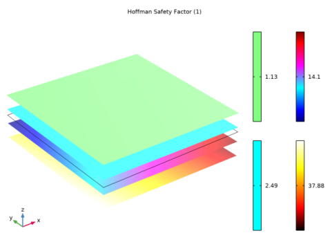
In the Settings window for 3D Plot Group, type Hoffman Safety Factors in Stack of Shells in the Label text field.
3
Locate the Title section. From the Title type list, choose Manual.
4
In the Title text area, type Hoffman Safety Factor (1).
Surface 1
1
Right-click Hoffman Safety Factors in Stack of Shells and choose Surface.
2
In the Settings window for Surface, locate the Expression section.
3
In the Expression text field, type shell1.emm1.sf3.s_fm.
Deformation 1
1
Right-click Surface 1 and choose Deformation.
2
In the Settings window for Deformation, locate the Expression section.
3
In the Z component text field, type w+1.5e-3.
4
Locate the Scale section. Select the Scale factor check box.
5
Surface 2, 3, 4
Create three similar Surface nodes by duplicating the above node, and replace the word shell1 in the Expression by shell2, shell3, and shell4 for Surface 2, Surface 3, and Surface 4, respectively. Replace the choice of color table in the subsequent Surface nodes, and also replace the Z component field in the corresponding Deformation node with the following choices in the table:
Hoffman Safety Factors in Stack of Shells
1
In the Model Builder window, click Hoffman Safety Factors in Stack of Shells.
2
In the Settings window for 3D Plot Group, locate the Color Legend section.
3
From the Position list, choose Right double.