PDF

Bracket — Transient Analysis
Introduction
Transient analyses provide the time domain response of a structure subjected to time-dependent loads. A transient analysis can be important when the time scale of the load is such that inertial or damping effects might have a significant influence on the behavior of the structure.
In this example you learn how to add damping properties to the material, define external loads varying with time, set up time-stepping data for the study, and generate animations.
It is recommended you review the Introduction to the Structural Mechanics Module, which includes background information and discusses the bracket_basic.mph models relevant to this example.
Model Definition
This model is an extension of the example described in the section “The Fundamentals: A Static Linear Analysis” in the Introduction to the Structural Mechanics Module.
The model geometry is represented in Figure 1.
Figure 1: Bracket geometry.
A rigid body is assumed to be connected to the arms of the bracket on which the time-varying load is applied. This body is modeled using a rigid connector.
Results and Discussion
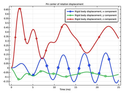
Figure 2 shows the rigid connector’s displacements at the center of rotation versus the time.
Figure 2: Displacement of the pin center of rotation vs time.
Notes About the COMSOL Implementation
To accurately model the physical problem, you need to apply damping in a dynamic analysis. In COMSOL you have the possibility to add damping of several types: isotropic loss factor, anisotropic loss factor, viscous damping, or Rayleigh damping.
To describe time-dependent boundary conditions you can enter expressions using the built-in variable t, the time variable in COMSOL Multiphysics.
The scaling of the displacement variables can be changed to correspond to the expected deformations. Manual scaling is the default for the displacement variables. The default manual scaling used for the structural displacement is 1% of the geometry size, which in this example is about 200 mm. In this case the expected deformations are in the order of 0.1 mm. The manual scaling factor should thus be changed to 10-4.
Application Library path: Structural_Mechanics_Module/Tutorials/bracket_transient
Modeling Instructions
From the File menu, choose Open.
Browse to the model’s Application Libraries folder and double-click the file bracket_basic.mph.
Solid Mechanics (solid)
Linear Elastic Material 1
In the Model Builder window, expand the Component 1 (comp1)>Solid Mechanics (solid) node, then click Linear Elastic Material 1.
Damping 1
1
In the Physics toolbar, click  Attributes and choose Damping.
In this example, you will use Rayleigh damping.
2
In the Settings window for Damping, locate the Damping Settings section.
3
In the αdM text field, type 50.
4
In the βdK text field, type 1e-4.
To represent the pin between the arms of the bracket you can use a rigid connector, to which a load is applied.
Rigid Connector 1
1
In the Physics toolbar, click  Boundaries and choose Rigid Connector.
2
In the Settings window for Rigid Connector, locate the Boundary Selection section.
3
From the Selection list, choose Pin Holes.
Applied Force 1
1
In the Physics toolbar, click  Attributes and choose Applied Force.
2
In the Settings window for Applied Force, locate the Applied Force section.
3
Specify the F vector as
Add Study
1
In the Home toolbar, click  Add Study to open the Add Study window.
2
Go to the Add Study window.
3
Find the Studies subsection. In the Select Study tree, select General Studies>Time Dependent.
4
Click Add Study in the window toolbar.
5
In the Home toolbar, click  Add Study to close the Add Study window.
Study 1
Step 1: Time Dependent
1
In the Settings window for Time Dependent, locate the Study Settings section.
2
From the Time unit list, choose ms.
3
In the Output times text field, type range(0,0.25,25).
With this time stepping, the solver automatically stores the solution every 0.25 ms from 0 to 25 ms.
The time-dependent solver adapts its time stepping based on a tolerance criterion. This ensures that the solver takes small enough time steps if large variations occur between the specified output times.
4
From the Tolerance list, choose User controlled.
5
In the Relative tolerance text field, type 0.001.
6
Click to expand the Results While Solving section. Select the Plot check box.
Solution 1 (sol1)
1
In the Study toolbar, click  Show Default Solver.
2
In the Model Builder window, expand the Solution 1 (sol1) node.
3
In the Model Builder window, expand the Study 1>Solver Configurations>Solution 1 (sol1)>Dependent Variables 1 node, then click Displacement field (comp1.u).
4
In the Settings window for Field, locate the Scaling section.
5
In the Scale text field, type 1e-4.
You can speed up the computation for a small model by disabling the convergence plot. To do this, go to the Options menu and select Preferences. Under Results, click to clear the Generate convergence plots check box.
6
In the Study toolbar, click  Compute.
Results
Stress (solid)
1
Click the  Zoom Extents button in the Graphics toolbar.
The default plot shows the stress distribution at the final time. You can change the time for the plot display in the Time list of the plot group settings.
Plot the displacement of the center of rotation of the rigid body versus the time.
1D Plot Group 3
1
In the Home toolbar, click  Add Plot Group and choose 1D Plot Group.
2
In the Settings window for 1D Plot Group, click to expand the Title section.
3
From the Title type list, choose Manual.
4
In the Title text area, type Pin center of rotation displacement.
5
Locate the Legend section. From the Position list, choose Upper left.
Global 1
1
Right-click 1D Plot Group 3 and choose Global.
2
In the Settings window for Global, locate the y-Axis Data section.
3
4
Click to expand the Legends section. Click to expand the Coloring and Style section. Find the Line markers subsection. From the Marker list, choose Cycle.
5
In the Width text field, type 3.
6
In the 1D Plot Group 3 toolbar, click  Plot.
1D Plot Group 3
1
In the Model Builder window, click 1D Plot Group 3.
2
In the Settings window for 1D Plot Group, locate the Legend section.
3
From the Position list, choose Upper right.
4
In the 1D Plot Group 3 toolbar, click  Plot.
To visualize the results in an animation, create a player.
Animation 1
1
In the Results toolbar, click  Animation and choose File.
2
In the Settings window for Animation, locate the Target section.
3
From the Target list, choose Player.
4
Locate the Frames section. From the Frame selection list, choose All.
5
Click  Show Frame.
COMSOL Multiphysics generates the movie and then plays it. To replay the movie, click the Play button in the Graphics toolbar.
If you want to export a movie in GIF, Flash, or AVI format, right-click Export and create an Animation node.