PDF

Bracket — Static Analysis
Introduction
The various examples based on a bracket geometry form a suite of tutorials which summarizes the fundamentals when modeling structural mechanics problems in COMSOL Multiphysics and the Structural Mechanics Module.
This is the most fundamental model in the suite, and includes the definition of material properties and boundary conditions. After the solution is computed, you learn how to analyze results and check the reaction forces.
Model Definition
The model used in this guide is a bracket made of steel. This type of bracket can be used to install an actuator that is mounted on a pin placed between the two holes in the bracket arms. The geometry is shown in Figure 1.
Figure 1: Bracket geometry.
In this analysis, the mounting bolts are assumed to be fixed and securely bonded to the bracket. One of the arms is loaded upward and the other downward. The loads are applied as a pressure on the inner surfaces of the holes, and their intensity is P0 cos(α), where α is the angle from the direction of the load resultants. Figure 2 below shows the loads applied to the bracket.
Figure 2: Load distribution in the bracket arms.
Results
Figure 3 shows the von Mises stress distribution together with an exaggerated (automatically scaled) picture of the deformation. The high stress values are located in the vicinity of the mounting bolts and at the transition between the plates.
Figure 3: Von Mises stress distribution in the bracket under bending load in z-axis direction.
In Figure 4 you can see that the bracket base remains fixed while only the arms are deformed. The maximum total displacement is about 0.2 mm, which is in agreement with the assumption of small deformations.
Figure 4: Total displacement.
Figure 5 shows the principal stresses in the bracket. The largest principal stress is shown with red arrows, the intermediate principal stress with green arrows, and the smallest principal stress with blue arrows.
Figure 5: Principal stress in the bracket left arm.
In Table 1 you can see the reaction force in the x, y, and z directions in each bolt. In all directions the sum is zero, which is a good check, since in this model there are no resultant forces. The slight asymmetry can be attributed to the mesh not being perfectly symmetric.
Application Library path: Structural_Mechanics_Module/Tutorials/bracket_static
Modeling Instructions
From the File menu, choose New.
New
In the New window, click  Model Wizard.
Model Wizard
1
In the Model Wizard window, The first step to build a model is to open COMSOL and then specify the type of analysis you want to do - in this case, a stationary, solid mechanics analysis.
2
3
In the Select Physics tree, select Structural Mechanics>Solid Mechanics (solid).
4
Click Add.
5
Click  Study.
6
In the Select Study tree, select General Studies>Stationary.
7
Global Definitions
It is good modeling practice to gather the constants and parameters in one place so that you can change them easily. Using parameters will also improve the readability of your input data.
Parameters 1
1
In the Model Builder window, under Global Definitions click Parameters 1.
2
In the Settings window for Parameters, locate the Parameters section.
3
Geometry 1
The next step is to create your geometry, which also can be imported from an external program. COMSOL Multiphysics supports a multitude of CAD programs and file formats. In this example, import a file in the COMSOL Multiphysics geometry file format (.mphbin).
Import 1 (imp1)
1
In the Home toolbar, click  Import.
2
In the Settings window for Import, locate the Import section.
3
From the Source list, choose COMSOL Multiphysics file.
4
Click Browse.
5
6
Click Import.
Block 1 (blk1)
It is possible to create a free tetrahedral mesh covering the whole component. Such a strategy is however not efficient for the large flat regions. For this reason, you will partition the geometry, so that you can create a better mesh.
1
In the Geometry toolbar, click  Block.
2
In the Settings window for Block, locate the Selections of Resulting Entities section.
3
Find the Cumulative selection subsection. Click New.
4
In the New Cumulative Selection dialog box, type Partition Block in the Name text field.
5
6
In the Settings window for Block, locate the Size and Shape section.
7
In the Width text field, type 0.025.
8
In the Depth text field, type 0.13.
9
In the Height text field, type 0.04.
10
Locate the Position section. In the x text field, type -0.11.
11
In the y text field, type -0.12.
12
In the z text field, type 0.025.
13
Click  Build Selected.
Mirror 1 (mir1)
1
In the Geometry toolbar, click  Transforms and choose Mirror.
2
In the Settings window for Mirror, locate the Input section.
3
From the Input objects list, choose Partition Block.
4
Select the Keep input objects check box.
5
Locate the Selections of Resulting Entities section. Find the Cumulative selection subsection. From the Contribute to list, choose Partition Block.
6
Click  Build Selected.
Mirror 2 (mir2)
1
In the Geometry toolbar, click  Transforms and choose Mirror.
2
In the Settings window for Mirror, locate the Input section.
3
From the Input objects list, choose Partition Block.
4
Select the Keep input objects check box.
5
Locate the Normal Vector to Plane of Reflection section. In the x text field, type 1.
6
In the z text field, type 0.
7
Locate the Selections of Resulting Entities section. Find the Cumulative selection subsection. From the Contribute to list, choose Partition Block.
8
Click  Build Selected.
Partition Objects 1 (par1)
1
In the Geometry toolbar, click  Booleans and Partitions and choose Partition Objects.
2
3
In the Settings window for Partition Objects, locate the Partition Objects section.
4
Find the Tool objects subsection. Select the  Activate Selection toggle button.
5
From the Tool objects list, choose Partition Block.
6
Click  Build Selected.
Form Union (fin)
1
In the Geometry toolbar, click  Build All.
2
Click the  Zoom Extents button in the Graphics toolbar.
Definitions
Here you want to define an expression for the load applied to the load-carrying holes. Assume the load distribution to be defined by a trigonometric function.
Analytic 1 (an1)
1
In the Home toolbar, click  Functions and choose Local>Analytic.
2
In the Settings window for Analytic, type load in the Function name text field.
3
Locate the Definition section. In the Expression text field, type F*cos(atan2(py,abs(px))).
4
In the Arguments text field, type F, py, px.
5
Locate the Units section. In the Arguments text field, type Pa, m, m.
6
In the Function text field, type Pa.
Bolt 1
1
In the Definitions toolbar, click  Explicit.
2
In the Settings window for Explicit, type Bolt 1 in the Label text field.
3
Click the  Wireframe Rendering button in the Graphics toolbar.
4
Locate the Input Entities section. From the Geometric entity level list, choose Boundary.
5
6
Select the Group by continuous tangent check box.
7
Bolt Holes
1
In the Definitions toolbar, click  Union.
2
In the Settings window for Union, type Bolt Holes in the Label text field.
3
Locate the Geometric Entity Level section. From the Level list, choose Boundary.
4
5
Locate the Input Entities section. Under Selections to add, click  Add.
6
In the Add dialog box, in the Selections to add list, choose Bolt 1, Bolt 2, Bolt 3, and Bolt 4.
7
Create selections for the two holes carrying the load.
Left Pin Hole
1
In the Definitions toolbar, click  Explicit.
2
In the Settings window for Explicit, type Left Pin Hole in the Label text field.
3
Locate the Input Entities section. From the Geometric entity level list, choose Boundary.
4
5
Select the Group by continuous tangent check box.
6
Right Pin Hole
1
In the Definitions toolbar, click  Explicit.
2
In the Settings window for Explicit, type Right Pin Hole in the Label text field.
3
Locate the Input Entities section. From the Geometric entity level list, choose Boundary.
4
5
Select the Group by continuous tangent check box.
6
Add a selection to be used during mesh generation.
Pin Holes
1
In the Definitions toolbar, click  Union.
2
In the Settings window for Union, type Pin Holes in the Label text field.
3
Locate the Geometric Entity Level section. From the Level list, choose Boundary.
4
Locate the Input Entities section. Under Selections to add, click  Add.
5
In the Add dialog box, in the Selections to add list, choose Left Pin Hole and Right Pin Hole.
6
Bolt Hole Edges
1
In the Definitions toolbar, click  Adjacent.
2
In the Settings window for Adjacent, type Bolt Hole Edges in the Label text field.
3
Locate the Input Entities section. From the Geometric entity level list, choose Boundary.
4
Locate the Output Entities section. From the Geometric entity level list, choose Adjacent edges.
5
Locate the Input Entities section. Under Input selections, click  Add.
6
In the Add dialog box, select Bolt Holes in the Input selections list.
7
8
Click the  Wireframe Rendering button in the Graphics toolbar.
Materials
COMSOL Multiphysics is equipped with built-in material properties for a number of common materials. Here, choose structural steel. The material is automatically assigned to all domains.
Add Material
1
In the Home toolbar, click  Add Material to open the Add Material window.
2
Go to the Add Material window.
3
In the tree, select Built-in>Structural steel.
4
Click Add to Component in the window toolbar.
5
In the Home toolbar, click  Add Material to close the Add Material window.
Solid Mechanics (solid)
By default, the Solid Mechanics interface assumes that the participating material models are linear elastic, which is appropriate for this example. All that is left to do is to define the constraints and loads.
Fixed Constraint 1
1
In the Model Builder window, under Component 1 (comp1) right-click Solid Mechanics (solid) and choose Fixed Constraint.
2
In the Settings window for Fixed Constraint, locate the Boundary Selection section.
3
From the Selection list, choose Bolt Holes.
Boundary Load 1
Apply a boundary load to the bracket holes. The predefined boundary system is used for orienting the load in the normal direction. Note how boolean expressions like Z>0 can be used to limit the part of the hole where the load is active. Also, the sign of the X-coordinate is used to flip where the load is applied.
1
In the Physics toolbar, click  Boundaries and choose Boundary Load.
2
In the Settings window for Boundary Load, locate the Boundary Selection section.
3
From the Selection list, choose Pin Holes.
4
Locate the Coordinate System Selection section. From the Coordinate system list, choose Boundary System 1 (sys1).
5
Locate the Force section. Specify the FA vector as
Mesh 1
Start by creating an edge mesh around the bolt holes to make sure that they are properly resolved.
Edge 1
1
In the Mesh toolbar, click  Boundary and choose Edge.
2
In the Settings window for Edge, locate the Edge Selection section.
3
From the Selection list, choose Bolt Hole Edges.
Distribution 1
1
Right-click Edge 1 and choose Distribution.
2
In the Settings window for Distribution, locate the Distribution section.
3
In the Number of elements text field, type 8.
Create a mesh which is swept through the thin flat parts, and then use a free tetrahedral mesh in the parts with a more complex geometry. Note that the transition between the two types of elements is automatic.
Swept 1
1
In the Mesh toolbar, click  Swept.
2
In the Settings window for Swept, locate the Domain Selection section.
3
From the Geometric entity level list, choose Domain.
4
5
Click to expand the Source Faces section. Select Boundaries 1, 33, 37, 50, and 72 only.
Size 1
1
Right-click Swept 1 and choose Size.
2
In the Settings window for Size, locate the Element Size section.
3
Click the Custom button.
4
Locate the Element Size Parameters section. Select the Maximum element size check box.
5
6
Click  Build Selected.
Free Tetrahedral 1
In the Mesh toolbar, click  Free Tetrahedral.
Size 1
1
Right-click Free Tetrahedral 1 and choose Size.
2
In the Settings window for Size, locate the Element Size section.
3
From the Predefined list, choose Finer.
4
Click  Build All.
The steps below show how to visualize the load distribution in the current geometry before computing the solution.
Study 1
In the Study toolbar, click  Get Initial Value.
Note that the Study node automatically defines a solver sequence for the simulation based on the selected physics (Solid Mechanics) and study type (Stationary).
Results
Boundary Loads (solid)
1
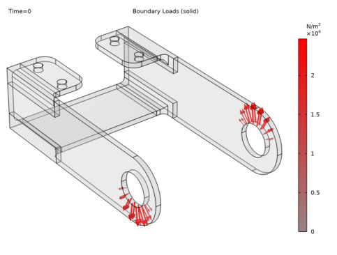
In the Model Builder window, expand the Results>Applied Loads (solid) node, then click Boundary Loads (solid).
2
In the Boundary Loads (solid) toolbar, click  Plot.
Now, solve the model.
Study 1
In the Home toolbar, click  Compute.
The default plot shows the von Mises stress distribution, together with an exaggerated (automatically scaled) picture of the deformation.
Results
Surface 1
1
In the Model Builder window, expand the Results>Stress (solid) node, then click Surface 1.
2
In the Settings window for Surface, locate the Expression section.
3
From the Unit list, choose MPa.
Boundary Load 1
1
In the Model Builder window, expand the Results>Applied Loads (solid)>Boundary Loads (solid) node.
2
Right-click Boundary Load 1 and choose Copy.
Boundary Load 1
1
In the Model Builder window, right-click Stress (solid) and choose Paste Arrow Surface.
2
In the Settings window for Arrow Surface, locate the Coloring and Style section.
3
From the Arrow base list, choose Head.
4
Select the Scale factor check box.
5
6
Click to expand the Inherit Style section. From the Plot list, choose Surface 1.
7
Clear the Arrow scale factor check box.
8
Clear the Color check box.
9
Clear the Color and data range check box.
Color Expression
1
In the Model Builder window, expand the Boundary Load 1 node, then click Color Expression.
2
In the Settings window for Color Expression, locate the Coloring and Style section.
3
Clear the Color legend check box.
4
Click the  Show Grid button in the Graphics toolbar.
5
Click the  Zoom Extents button in the Graphics toolbar.
Add a plot group to display the displacement of the bracket.
Total Displacement
1
In the Home toolbar, click  Add Plot Group and choose 3D Plot Group.
2
In the Settings window for 3D Plot Group, type Total Displacement in the Label text field.
Surface 1
1
Right-click Total Displacement and choose Surface.
2
In the Settings window for Surface, locate the Expression section.
3
From the Unit list, choose mm.
4
Locate the Coloring and Style section. From the Color table list, choose Cividis.
Marker 1
1
Right-click Surface 1 and choose Marker.
2
In the Settings window for Marker, locate the Display section.
3
From the Display list, choose Max.
4
Locate the Coloring and Style section. From the Background color list, choose From theme.
5
Locate the Text Format section. In the Display precision text field, type 2.
Total Displacement
1
In the Model Builder window, click Total Displacement.
2
In the Settings window for 3D Plot Group, locate the Color Legend section.
3
From the Position list, choose Bottom.
4
In the Total Displacement toolbar, click  Plot.
Create another plot to display the principal stresses.
Principal Stress
1
In the Home toolbar, click  Add Plot Group and choose 3D Plot Group.
2
In the Settings window for 3D Plot Group, type Principal Stress in the Label text field.
Principal Stress Volume 1
1
In the Principal Stress toolbar, click  More Plots and choose Principal Stress Volume.
2
In the Settings window for Principal Stress Volume, locate the Positioning section.
3
Find the X grid points subsection. In the Points text field, type 30.
4
Find the Y grid points subsection. In the Points text field, type 60.
5
Find the Z grid points subsection. In the Points text field, type 15.
6
Locate the Coloring and Style section. From the Arrow length list, choose Logarithmic.
7
In the Principal Stress toolbar, click  Plot.
A final check is to compute the total reaction force along the x-, y-, and z-directions. Use a surface integration over the constrained boundaries.
Evaluation Group: Reactions
1
In the Results toolbar, click  Evaluation Group.
2
In the Settings window for Evaluation Group, type Evaluation Group: Reactions in the Label text field.
Bolt 1
1
Right-click Evaluation Group: Reactions and choose Integration>Surface Integration.
2
In the Settings window for Surface Integration, type Bolt 1 in the Label text field.
3
Locate the Selection section. From the Selection list, choose Bolt 1.
4
Click Replace Expression in the upper-right corner of the Expressions section. From the menu, choose Component 1 (comp1)>Solid Mechanics>Reactions>Reaction force (spatial frame) - N>All expressions in this group.
5
Locate the Expressions section. In the table, enter the following settings:
Bolt 2
1
Right-click Bolt 1 and choose Duplicate.
2
In the Settings window for Surface Integration, type Bolt 2 in the Label text field.
3
Locate the Selection section. From the Selection list, choose Bolt 2.
4
Locate the Expressions section. In the table, enter the following settings:
Bolt 3
1
Right-click Bolt 2 and choose Duplicate.
2
In the Settings window for Surface Integration, type Bolt 3 in the Label text field.
3
Locate the Selection section. From the Selection list, choose Bolt 3.
4
Locate the Expressions section. In the table, enter the following settings:
Bolt 4
1
Right-click Bolt 3 and choose Duplicate.
2
In the Settings window for Surface Integration, type Bolt 4 in the Label text field.
3
Locate the Selection section. From the Selection list, choose Bolt 4.
4
Locate the Expressions section. In the table, enter the following settings:
5
In the Evaluation Group: Reactions toolbar, click  Evaluate.