|
|
|
|
1
|
|
2
|
|
3
|
Click Add.
|
|
4
|
|
5
|
Click Add.
|
|
6
|
|
7
|
Click
|
|
8
|
|
9
|
Click
|
|
1
|
|
2
|
|
3
|
|
4
|
Browse to the model’s Application Libraries folder and double-click the file block_on_arch_parameters.txt.
|
|
1
|
|
2
|
|
3
|
|
4
|
|
1
|
|
2
|
|
3
|
|
4
|
|
5
|
|
6
|
|
7
|
|
8
|
|
9
|
|
1
|
|
2
|
On the object c1, select Boundaries 2 and 3 only.
|
|
1
|
|
2
|
On the object del1, select Boundary 1 only.
|
|
1
|
|
2
|
|
3
|
|
4
|
|
5
|
|
6
|
|
7
|
|
8
|
|
1
|
|
2
|
|
3
|
|
4
|
|
5
|
|
6
|
|
1
|
|
2
|
|
1
|
|
2
|
|
3
|
|
1
|
|
2
|
|
4
|
|
5
|
|
1
|
|
2
|
|
3
|
|
4
|
Select the object ext1(1) only.
|
|
5
|
|
6
|
|
1
|
|
2
|
|
3
|
|
4
|
Select the object ext1(2) only.
|
|
5
|
|
1
|
|
2
|
|
3
|
|
4
|
|
5
|
|
1
|
In the Model Builder window, under Component 1 (comp1) right-click Materials and choose Blank Material.
|
|
2
|
|
1
|
|
2
|
|
3
|
|
4
|
|
5
|
|
1
|
|
2
|
|
3
|
|
1
|
|
2
|
|
3
|
|
1
|
|
2
|
|
1
|
|
3
|
|
4
|
|
5
|
|
1
|
|
2
|
|
3
|
|
1
|
|
2
|
|
3
|
|
4
|
|
5
|
|
1
|
|
3
|
In the Settings window for Prescribed Displacement/Rotation, locate the Prescribed Displacement section.
|
|
4
|
|
5
|
|
6
|
|
1
|
|
1
|
|
2
|
|
3
|
|
4
|
|
5
|
Click OK.
|
|
6
|
|
7
|
|
8
|
|
1
|
|
3
|
|
4
|
|
1
|
|
1
|
|
3
|
|
4
|
|
5
|
|
6
|
In the Show More Options dialog box, in the tree, select the check box for the node Physics>Equation-Based Contributions.
|
|
7
|
Click OK.
|
|
1
|
|
2
|
|
4
|
|
5
|
|
6
|
Click
|
|
7
|
|
8
|
Click OK.
|
|
1
|
|
2
|
|
3
|
|
4
|
|
1
|
|
2
|
|
3
|
|
1
|
|
3
|
|
4
|
|
1
|
|
1
|
|
3
|
|
4
|
|
1
|
|
1
|
|
2
|
|
3
|
|
1
|
|
2
|
|
3
|
|
4
|
Click
|
|
1
|
|
2
|
|
3
|
|
4
|
|
5
|
In the Model Builder window, expand the Study 1>Solver Configurations>Solution 1 (sol1)>Dependent Variables 1 node, then click State variable load (comp1.ODE1).
|
|
6
|
|
7
|
|
8
|
In the Model Builder window, expand the Study 1>Solver Configurations>Solution 1 (sol1)>Stationary Solver 1>Segregated 1 node, then click Shell.
|
|
9
|
|
10
|
|
11
|
|
12
|
Click OK.
|
|
13
|
In the Model Builder window, under Study 1>Solver Configurations>Solution 1 (sol1)>Stationary Solver 1>Segregated 1 right-click Solid Mechanics and choose Delete.
|
|
14
|
|
1
|
|
2
|
|
3
|
|
4
|
|
5
|
|
6
|
|
7
|
|
8
|
|
9
|
|
10
|
|
1
|
|
2
|
|
3
|
|
1
|
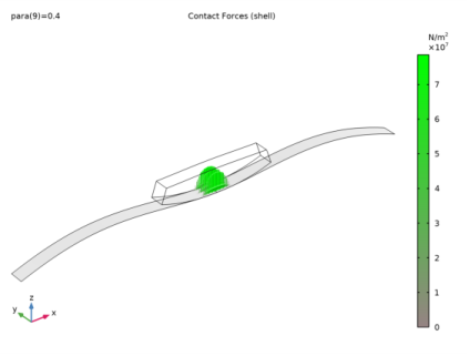
In the Model Builder window, expand the Contact Forces (shell) node, then click Contact 1, Pressure.
|
|
2
|
|
3
|
|
4
|
|
1
|
In the Model Builder window, expand the Results>Contact Forces (shell)>Gray Surfaces node, then click Selection 1.
|
|
3
|
|
4
|
|
5
|
|
1
|
|
2
|
|
3
|
|
4
|
|
1
|
|
2
|
|
1
|
|
2
|
|
4
|
|
5
|
|
6
|
Click to expand the Coloring and Style section. Find the Line markers subsection. From the Marker list, choose Cycle.
|
|
1
|
|
2
|
|
3
|
|
4
|
|
5
|
|
6
|
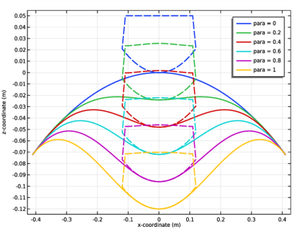
In the associated text field, type Deflection (mm).
|
|
7
|
|
1
|
|
2
|
|
3
|
|
4
|
|
5
|
|
1
|
|
3
|
|
4
|
|
5
|
|
6
|
|
7
|
|
1
|
|
2
|
|
3
|
|
5
|
Locate the Coloring and Style section. Find the Line style subsection. From the Line list, choose Dashed.
|
|
6
|
|
1
|
|
2
|
|
3
|
|
4
|
|
5
|