PDF

Wave Propagation in Rock Under Blast Loads
Introduction
This example presents a transient analysis of the wave propagation in a rock mass caused by a short duration load on the surface. Such loads are typical during tunnel constructions and other excavations using blasting. It shows the use of the Low-reflecting boundary conditions to truncate the computational domain to a reasonable size. The results are in very good agreement with a published study, Ref. 1.
As a default, the low-reflecting boundary condition takes the material data from the adjacent domain in an attempt to create a perfect impedance match for both pressure waves and shear waves, so that
where n and t are the unit normal and tangential vectors at the boundary, respectively, and cp and cs are the speeds of the pressure and shear waves in the material. This approach works best when the wave direction in close to the normal at the wall.
More information about modeling using low-reflecting boundary conditions can be found in Ref. 2.
Model Definition
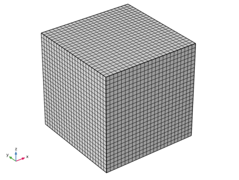
The model geometry is a block. Two of the side walls are symmetry planes. The other two represent the truncation of the computational domain in the directions where the rock has lateral dimensions that are significantly larger than the depth. The size of the block and the material parameters correspond to that studied in Ref. 1.
Figure 1: Geometry and mesh.
Thus, the following elastic material data is used: the Young’s modulus E =  50 GPa, Poisson’s ratio ν =  2/7, and density ρ = 2700 kg/m3. These values represent a granite rock.
The upper surface is free, and the bottom surface is subjected to loading in form of a finite duration pressure pulse localized near the origin, see Figure 2. The loading is similar to that used in Ref. 1 and represents an explosion within the rock near the surface.
The truncation boundaries are modeled with, and then without, applying the low-reflecting boundary conditions.
Figure 2: The load function.
Results and Discussion
The wave propagation in the block is modeled via a transient study covering a time interval of 150 ms. The typical wave propagation pattern is shown in Figure 3.
The vertical displacement at the upper surface is shown in Figure 4 for both cases, with and without using the low-reflecting boundary conditions. The analytical estimate for the time when the pressure wave reaches the surface is H/cp, where H is the height of the block. In case of reflection, the time for the reflected pressure wave to arrive at the sampling point is , where L is the distance of blast point from the truncated boundaries. Both estimates have very good agreement with the computations. Thus, the two responses start to deviate from each other after the estimated time as shown in Figure 4, which is caused by the reflected wave.
Figure 3: The stress in the block at the early stage of the elastic wave propagation.
Figure 4: The displacement at the upper surface for the cases with (solid line) and without (dotted line) applying the low-reflecting boundary conditions. The dashed vertical lines represent analytical estimates for time of arrival of incoming and reflected waves, respectively.
References
1. H. Sönnerlind, “Beräkningsmetoder för spänningar i explosionsbelastad berg,” rapport nr 001202 (in Swedish), Epsilon HighTech Innovation AB, 2005.
2. M. Cohen and P.C. Jennings, “Silent Boundary Methods for Transient Analysis,” Computational Methods for Transient Analysis, vol. 1, T. Belytschko and T.J.R. Hughes, eds., North-Holland, 1983.
Application Library path: Structural_Mechanics_Module/Elastic_Waves/blasting_rock
Modeling Instructions
From the File menu, choose New.
New
In the New window, click  Model Wizard.
Model Wizard
1
In the Model Wizard window, click  3D.
2
In the Select Physics tree, select Structural Mechanics>Solid Mechanics (solid).
3
Click Add.
4
Click  Study.
5
In the Select Study tree, select General Studies>Time Dependent.
6
Global Definitions
Define the geometry and loading parameters.
Parameters 1
1
In the Model Builder window, under Global Definitions click Parameters 1.
2
In the Settings window for Parameters, locate the Parameters section.
3
Definitions
Next, define the loading function.
Piecewise 1 (pw1)
1
In the Home toolbar, click  Functions and choose Local>Piecewise.
2
In the Settings window for Piecewise, type Pb in the Function name text field.
3
Locate the Definition section. In the Argument text field, type t.
4
Find the Intervals subsection. In the table, enter the following settings:
5
Locate the Units section. In the Arguments text field, type s.
6
In the Function text field, type N.
Plot the function which should look similar to that shown in Figure 2.
7
Geometry 1
Block 1 (blk1)
1
In the Geometry toolbar, click  Block.
2
In the Settings window for Block, locate the Size and Shape section.
3
In the Width text field, type L.
4
In the Depth text field, type L.
5
In the Height text field, type H.
6
Click  Build Selected.
7
In the Geometry toolbar, click  Build All.
Enter the material parameters, which correspond to granite rock.
Solid Mechanics (solid)
Linear Elastic Material 1
1
In the Model Builder window, under Component 1 (comp1)>Solid Mechanics (solid) click Linear Elastic Material 1.
2
In the Settings window for Linear Elastic Material, locate the Linear Elastic Material section.
3
From the E list, choose User defined. In the associated text field, type 50[GPa].
4
From the ν list, choose User defined. In the associated text field, type 2/7.
5
From the ρ list, choose User defined. In the associated text field, type 2700.
Beacause of the symmetry, you model one quarter of the geometry. This also explains the factor of 0.25 used in the load expression, since the load is given as a total force.
Symmetry 1
1
In the Physics toolbar, click  Boundaries and choose Symmetry.
2
Boundary Load 1
1
In the Physics toolbar, click  Boundaries and choose Boundary Load.
2
3
In the Settings window for Boundary Load, locate the Force section.
4
Specify the FA vector as
Low-Reflecting Boundary 1
1
In the Physics toolbar, click  Boundaries and choose Low-Reflecting Boundary.
2
Use linear elements to reduce the numerical dispersion of the wavefront.
3
In the Model Builder window, click Solid Mechanics (solid).
4
In the Settings window for Solid Mechanics, click to expand the Discretization section.
5
From the Displacement field list, choose Linear.
Mesh 1
Mapped 1
1
In the Mesh toolbar, click  Boundary and choose Mapped.
2
The number of elements in the Distribution node should be written as floor(L/L1) in order to have the input in an integer format.
Distribution 1
1
Right-click Mapped 1 and choose Distribution.
2
3
In the Settings window for Distribution, locate the Distribution section.
4
In the Number of elements text field, type floor(L/L1).
5
Click  Build Selected.
Swept 1
In the Mesh toolbar, click  Swept.
Distribution 1
1
Right-click Swept 1 and choose Distribution.
2
In the Settings window for Distribution, locate the Distribution section.
3
In the Number of elements text field, type floor(L/L1).
4
In the Model Builder window, right-click Mesh 1 and choose Build All.
5
Click the  Go to Default View button in the Graphics toolbar.
The resulting mesh should be similar to that shown in Figure 1.
Study 1
Step 1: Time Dependent
1
In the Model Builder window, under Study 1 click Step 1: Time Dependent.
2
In the Settings window for Time Dependent, locate the Study Settings section.
3
In the Output times text field, type range(0,2e-6,1.5e-4).
Solution 1 (sol1)
1
In the Study toolbar, click  Show Default Solver.
2
In the Model Builder window, expand the Solution 1 (sol1) node.
The default scale for the displacement is based on the size of the geometry. Change this to a scale more suitable for the wave propagation analysis.
3
In the Model Builder window, expand the Study 1>Solver Configurations>Solution 1 (sol1)>Dependent Variables 1 node, then click Displacement field (comp1.u).
4
In the Settings window for Field, locate the Scaling section.
5
In the Scale text field, type u0.
6
In the Model Builder window, click Time-Dependent Solver 1.
7
In the Settings window for Time-Dependent Solver, click to expand the Time Stepping section.
8
In the Amplification for high frequency text field, type 0.5.
This change in the damping will help to suppress numerical artifacts in the transient solution.
Results
Before solving the problem, prepare a plot of the vertical displacement component. This will be shown and updated during the computations.
Displacement
1
In the Home toolbar, click  Add Plot Group and choose 1D Plot Group.
2
In the Settings window for 1D Plot Group, type Displacement in the Label text field.
3
Click to expand the Title section. From the Title type list, choose None.
Point Graph 1
1
Right-click Displacement and choose Point Graph.
2
3
In the Settings window for Point Graph, locate the y-Axis Data section.
4
In the Expression text field, type w.
5
In the Unit field, type um.
Study 1
Step 1: Time Dependent
1
In the Model Builder window, under Study 1 click Step 1: Time Dependent.
2
In the Settings window for Time Dependent, click to expand the Results While Solving section.
3
Select the Plot check box.
4
In the Home toolbar, click  Compute.
Results
Add a volume plot of the stress similar to that shown in Figure 3.
3D Plot Group 2
In the Home toolbar, click  Add Plot Group and choose 3D Plot Group.
Volume 1
1
Right-click 3D Plot Group 2 and choose Volume.
2
In the Settings window for Volume, locate the Expression section.
3
In the Expression text field, type solid.sz.
Deformation 1
Right-click Volume 1 and choose Deformation.
3D Plot Group 2
1
In the Settings window for 3D Plot Group, locate the Data section.
2
From the Time (s) list, choose 5E-5.
3
Click the  Transparency button in the Graphics toolbar.
4
In the 3D Plot Group 2 toolbar, click  Plot.
Isosurface 1
1
Right-click 3D Plot Group 2 and choose Isosurface.
2
In the Settings window for Isosurface, locate the Expression section.
3
In the Expression text field, type w.
Deformation 1
1
Right-click Isosurface 1 and choose Deformation.
2
In the 3D Plot Group 2 toolbar, click  Plot.
3
Click the  Go to Default View button in the Graphics toolbar.
Root
Next, add a new study, for which the low-reflecting boundary conditions will be disabled.
Add Study
1
In the Home toolbar, click  Add Study to open the Add Study window.
2
Go to the Add Study window.
3
Find the Studies subsection. In the Select Study tree, select General Studies>Time Dependent.
4
Click Add Study in the window toolbar.
5
In the Home toolbar, click  Add Study to close the Add Study window.
Study 2
Step 1: Time Dependent
1
In the Settings window for Time Dependent, locate the Study Settings section.
2
In the Output times text field, type range(0,2e-6,1.5e-4).
3
Locate the Results While Solving section. Select the Plot check box.
4
Locate the Physics and Variables Selection section. Select the Modify model configuration for study step check box.
5
In the Physics and variables selection tree, select Component 1 (comp1)>Solid Mechanics (solid)>Low-Reflecting Boundary 1.
6
Click  Disable.
7
In the Model Builder window, click Study 2.
8
In the Settings window for Study, locate the Study Settings section.
9
Clear the Generate default plots check box.
Configure the solver in the same way as for the first study
Solution 2 (sol2)
1
In the Study toolbar, click  Show Default Solver.
2
In the Model Builder window, expand the Solution 2 (sol2) node.
3
In the Model Builder window, expand the Study 2>Solver Configurations>Solution 2 (sol2)>Dependent Variables 1 node, then click Displacement field (comp1.u).
4
In the Settings window for Field, locate the Scaling section.
5
In the Scale text field, type u0.
6
In the Model Builder window, click Time-Dependent Solver 1.
7
In the Settings window for Time-Dependent Solver, locate the Time Stepping section.
8
In the Amplification for high frequency text field, type 0.5.
Results
Point Graph 2
1
In the Model Builder window, under Results>Displacement right-click Point Graph 1 and choose Duplicate.
2
In the Settings window for Point Graph, locate the Data section.
3
From the Dataset list, choose Study 2/Solution 2 (sol2).
4
Click to expand the Coloring and Style section. Find the Line style subsection. From the Line list, choose Dotted.
Study 2
In the Study toolbar, click  Compute.
Results
Displacement
Add the following line plots to show the estimated times at which the incoming and reflected pressure waves hit the block surface.
Point Graph 3
1
In the Model Builder window, right-click Displacement and choose Point Graph.
2
In the Settings window for Point Graph, locate the y-Axis Data section.
3
In the Expression text field, type (t/t0-1)*40.
4
Locate the x-Axis Data section. From the Parameter list, choose Expression.
5
In the Expression text field, type L/solid.cp.
6
7
Locate the Coloring and Style section. Find the Line style subsection. From the Line list, choose Dashed.
8
From the Color list, choose Red.
Point Graph 4
1
Right-click Point Graph 3 and choose Duplicate.
2
In the Settings window for Point Graph, locate the x-Axis Data section.
3
In the Expression text field, type L*sqrt(5)/solid.cp.
Displacement
1
In the Model Builder window, click Displacement.
2
In the Settings window for 1D Plot Group, locate the Plot Settings section.
3
Select the x-axis label check box.
4
5
Select the y-axis label check box.
6
In the associated text field, type Vertical displacement (um).
7
In the Displacement toolbar, click  Plot.
The final plot should look similar to that shown in Figure 4.