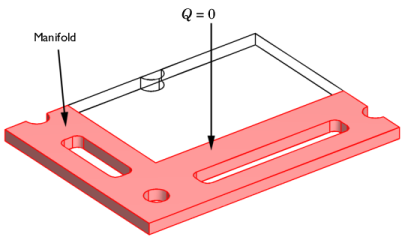
PDF

Fuel Cell Bipolar Plate
Introduction
This study presents a model that couples the thermal and the structural analysis in a bipolar plate in a proton exchange membrane fuel cell (PEMFC). The fuel cell stack consists of unit cell of anode, membrane, and cathode connected in series through bipolar plates. The bipolar plates also serve as gas distributors for hydrogen and air that is fed to the anode and cathode compartments, respectively. Figure 1 below shows a schematic drawing of a fuel cell stack. The unit cell and the surrounding bipolar plates are shown in detail in the upper right corner of the figure.
Figure 1: Schematic drawing of the fuel cell stack. The unit cell consists of an anode, membrane electrolyte, and a cathode. The unit cell is supported and supplied with reactants through the bipolar plates. The bipolar plates also serve as current collectors and feeders.
The PEMFC is one of the strongest alternatives for automotive applications where it has the potential of delivering power to a vehicle with a higher efficiency, from oil to propulsion, than the internal combustion engine.
The fuel cell operates at temperatures just below 100°C, which means that it has to be heated at startup. The heating process induces thermal stresses in the bipolar plates. This analysis reveals the magnitude and nature of these stresses.
Model Definition
Figure 2 below shows the detailed model geometry. The plate consists of gas slits that form the gas channels in the cell, holes for the tie rods that keep the stack together, and the heating elements, which are positioned in the middle of the gas feeding channel for the electrodes. Due to symmetry, it is possible to reduce the model geometry to 1/8 of the actual size of the cell.
Figure 2: The modeled geometry.
The study consists of a thermal-structural analysis. In the following specification of the problem a number of constants are used; their values are listed in the following table. The constant Q1 represents a power of 200 W distributed over the hole through the 25 bipolar plates in the fuel cell stack.
R0
Q1
200/(25·π·R0^2·th) W/m3
P1
P2
h1
5 W/(m2·K)
h2
50W/(m2·K)
Thermal Analysis
The general equation is the steady-state heat equation according to:
where k denotes the thermal conductivity of the different materials, T the temperature, and Q a heat source or heat sink.
The modeled domain consists of three different domains. The first domain corresponds to the active part of the cell, where the electric energy is produced and the current is conducted. The production and conduction of current involve some losses. It is assumed that the cell is heated prior to operation. This means that the model does not account for the heat sources due to the production and conduction of current; see Figure 3.
Figure 3: The active part of the cell bipolar plate is made of titanium.
The second domain corresponds to the heating element in the bipolar plate, which is made of aluminum. The power from this element is assumed to be uniformly distributed in the small cylindrical domain; see Figure 4.
Figure 4: The heating element in the bipolar plate is made of aluminum.
The last domain forms the manifold in the cell and it is made of titanium. In this domain, only heat conduction is present.
Figure 5: The domain that forms the manifold of the cell.
There are different material models present for both titanium and aluminum.
The boundary conditions for the heat transfer analysis are symmetry conditions and convective conditions. The symmetry condition states that the flux is zero through the boundary.
The convective conditions set the heat flux proportional to the temperature difference between the fluid outside and the temperature at the boundary. The heat transfer coefficient is the proportionality constant:
In this equation, h denotes the heat transfer coefficient.
Figure 6 shows the symmetry boundaries.
Figure 6: Symmetry boundaries.
Figure 7 shows the convective boundaries. The heat transfer coefficient is different for the different groups of boundaries in the figure.
Figure 7: The convective boundaries.
Structural Analysis
The thermal expansion causes the stresses in the domain. The thermal loads are proportional to the temperature difference between the reference state and the actual temperature.
The constrains are imposed on the symmetry planes, see Figure 8 and Figure 9. There the displacements perpendicular to the boundary are set to zero.
Figure 8: The symmetry boundaries.
Figure 9: Additional symmetry plane.
In addition, the load applied by the tie rods on the stack is applied in the manifold and the active part at the bipolar plate. The pressure is different in these two domains, see Figure 10.
The loads and constraints on all other boundaries are assumed to be negligible. In this context, the only questionable assumption is the possible loads and constraints imposed by the tie rods on the holes in the bipolar plate. In a more detailed analysis, it would be possible to couple a model for the tie rods with a detailed model of the bipolar plate. The probably the pressure on those different parts would show different gradients.
Figure 10: Pressure due to the rod connection.
Results
Figure 11 shows the temperature field at steady state. The slits for the gas present the largest sinks of heat at the boundaries. The temperature decreases almost with the radial distance from the heating element.
Figure 11: Temperature distribution in the plate.
Figure 12 shows that the thermal loads generate stresses that are one order of magnitude larger than those generated by the external pressure loads (which you can compute by turning off the thermal expansion). The loads are far from the critical values, but the displacements can be even more important. The displacements must be small enough to grant that the membrane can fulfill its function in separating hydrogen and oxygen in the anode and cathode compartments, respectively. The z-component of the displacement in shown in Figure 13.
Figure 12: Effective von Mises stresses due to temperature and external loads.
Figure 13: Expansion in the z direction.
Application Library path: Structural_Mechanics_Module/Thermal-Structure_Interaction/bipolar_plate
Modeling Instructions
From the File menu, choose New.
New
In the New window, click  Model Wizard.
Model Wizard
1
In the Model Wizard window, click  3D.
2
In the Select Physics tree, select Structural Mechanics>Thermal-Structure Interaction>Thermal Stress, Solid.
3
Click Add.
4
Click  Study.
5
In the Select Study tree, select General Studies>Stationary.
6
Geometry 1
The geometry sequence for the model is available in a file. If you want to create it from scratch yourself, you can follow the instructions in the Appendix — Geometry Modeling Instructions section. Otherwise, insert the geometry sequence as follows:
1
In the Geometry toolbar, click  Insert Sequence.
2
3
In the Geometry toolbar, click  Build All.
Fill the table with nongeometric parameters.
Global Definitions
Parameters 1
1
In the Model Builder window, under Global Definitions click Parameters 1.
2
In the Settings window for Parameters, locate the Parameters section.
3
Definitions
Create an Explicit selection of the boundaries for Symmetry features in both physics.
Symmetry
1
In the Definitions toolbar, click  Explicit.
2
In the Settings window for Explicit, type Symmetry in the Label text field.
3
Locate the Input Entities section. From the Geometric entity level list, choose Boundary.
4
It might be easier to select the correct boundaries by using the Selection List window. To open this window, in the Home toolbar click Windows and choose Selection List. (If you are running the cross-platform desktop, you find Windows in the main menu.)
Solid Mechanics (solid)
1
In the Model Builder window, under Component 1 (comp1) click Solid Mechanics (solid).
2
Materials
Titanium
1
In the Model Builder window, under Component 1 (comp1) right-click Materials and choose Blank Material.
2
3
In the Settings window for Material, locate the Material Contents section.
4
5
In the Label text field, type Titanium.
Aluminum
1
Right-click Materials and choose Blank Material.
2
3
In the Settings window for Material, locate the Material Contents section.
4
5
In the Label text field, type Aluminum.
Multiphysics
Thermal Expansion 1 (te1)
The reference temperature is taken from the Default Model Inputs node. You can modify it manually.
1
In the Model Builder window, under Component 1 (comp1)>Multiphysics click Thermal Expansion 1 (te1).
2
In the Settings window for Thermal Expansion, locate the Model Input section.
3
Click  Go to Source.
Global Definitions
Default Model Inputs
1
In the Model Builder window, under Global Definitions click Default Model Inputs.
2
In the Settings window for Default Model Inputs, locate the Browse Model Inputs section.
3
Find the Expression for remaining selection subsection. In the Volume reference temperature text field, type 0[degC].
Solid Mechanics (solid)
Symmetry 1
1
In the Physics toolbar, click  Boundaries and choose Symmetry.
2
In the Settings window for Symmetry, locate the Boundary Selection section.
3
From the Selection list, choose Symmetry.
Boundary Load 1
1
In the Physics toolbar, click  Boundaries and choose Boundary Load.
2
3
In the Settings window for Boundary Load, locate the Force section.
4
From the Load type list, choose Pressure.
5
In the p text field, type P1.
Boundary Load 2
1
In the Physics toolbar, click  Boundaries and choose Boundary Load.
2
3
In the Settings window for Boundary Load, locate the Force section.
4
From the Load type list, choose Pressure.
5
In the p text field, type P2.
Heat Transfer in Solids (ht)
In the Model Builder window, under Component 1 (comp1) click Heat Transfer in Solids (ht).
Symmetry 1
1
In the Physics toolbar, click  Boundaries and choose Symmetry.
2
In the Settings window for Symmetry, locate the Boundary Selection section.
3
From the Selection list, choose Symmetry.
Heat Source 1
1
In the Physics toolbar, click  Domains and choose Heat Source.
2
3
In the Settings window for Heat Source, locate the Heat Source section.
4
In the Q0 text field, type 200[W]/N/(pi*R0^2*th).
Heat Flux 1
1
In the Physics toolbar, click  Boundaries and choose Heat Flux.
2
3
In the Settings window for Heat Flux, locate the Heat Flux section.
4
Click the Convective heat flux button.
5
In the h text field, type 50.
6
In the Text text field, type 80[degC].
Heat Flux 2
1
In the Physics toolbar, click  Boundaries and choose Heat Flux.
2
3
In the Settings window for Heat Flux, locate the Heat Flux section.
4
Click the Convective heat flux button.
5
In the h text field, type 5.
6
In the Text text field, type 20[degC].
Mesh 1
Free Triangular 1
1
In the Mesh toolbar, click  Boundary and choose Free Triangular.
2
3
In the Settings window for Free Triangular, click  Build All.
Swept 1
In the Mesh toolbar, click  Swept.
Distribution 1
1
Right-click Swept 1 and choose Distribution.
2
In the Settings window for Distribution, locate the Distribution section.
3
In the Number of elements text field, type 3.
4
In the Model Builder window, right-click Mesh 1 and choose Build All.
Study 1
In the Home toolbar, click  Compute.
Results
Stress (solid)
The first default plot, displayed in Figure 12 shows the von Mises stress.
Surface 1
1
In the Model Builder window, expand the Stress (solid) node, then click Surface 1.
2
In the Settings window for Surface, locate the Expression section.
3
From the Unit list, choose MPa.
Deformation
1
In the Model Builder window, expand the Surface 1 node.
2
Right-click Deformation and choose Delete.
Surface 1
1
In the Model Builder window, click Surface 1.
2
In the Stress (solid) toolbar, click  Plot.
A group showing boundary loads is also added by default. The next default plot shows the temperature field which should be similar to that displayed in Figure 11.
Copy this plot and modify it to visualize the z-displacement field in the deformed plate as shown in Figure 13.
Displacement
1
In the Model Builder window, right-click Temperature (ht) and choose Duplicate.
2
In the Settings window for 3D Plot Group, type Displacement in the Label text field.
Surface
1
In the Model Builder window, expand the Displacement node, then click Surface.
2
In the Settings window for Surface, locate the Coloring and Style section.
3
From the Color table list, choose Rainbow.
4
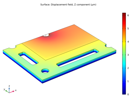
Click Replace Expression in the upper-right corner of the Expression section. From the menu, choose Component 1 (comp1)>Solid Mechanics>Displacement>Displacement field - m>w - Displacement field, Z component.
5
Locate the Expression section. From the Unit list, choose µm.
6
In the Displacement toolbar, click  Plot.
Appendix — Geometry Modeling Instructions
From the File menu, choose New.
New
In the New window, click  Model Wizard.
Model Wizard
1
In the Model Wizard window, click  3D.
2
In the Select Physics tree, select Structural Mechanics>Thermal-Structure Interaction>Thermal Stress, Solid.
3
Click Add.
4
Click  Study.
5
In the Select Study tree, select General Studies>Stationary.
6
Global Definitions
Parameters 1
1
In the Model Builder window, under Global Definitions click Parameters 1.
2
In the Settings window for Parameters, locate the Parameters section.
3
Geometry 1
Work Plane 1 (wp1)
1
In the Geometry toolbar, click  Work Plane.
2
In the Settings window for Work Plane, click  Show Work Plane.
Work Plane 1 (wp1)>Plane Geometry
In the Model Builder window, click Plane Geometry.
Work Plane 1 (wp1)>Rectangle 1 (r1)
1
In the Work Plane toolbar, click  Rectangle.
2
In the Settings window for Rectangle, locate the Size and Shape section.
3
In the Width text field, type 0.12.
4
In the Height text field, type 0.09.
5
Click  Build Selected.
6
Click the  Zoom Extents button in the Graphics toolbar.
Work Plane 1 (wp1)>Rectangle 2 (r2)
1
In the Work Plane toolbar, click  Rectangle.
2
In the Settings window for Rectangle, locate the Size and Shape section.
3
In the Width text field, type 0.09.
4
In the Height text field, type 0.055.
5
Locate the Position section. In the xw text field, type 0.03.
6
In the yw text field, type 0.035.
7
Click  Build Selected.
Work Plane 1 (wp1)>Rectangle 3 (r3)
1
In the Work Plane toolbar, click  Rectangle.
2
In the Settings window for Rectangle, locate the Size and Shape section.
3
In the Width text field, type 0.01.
4
In the Height text field, type 0.035.
5
Locate the Position section. In the xw text field, type 0.01.
6
In the yw text field, type 0.035.
7
Click  Build Selected.
Work Plane 1 (wp1)>Rectangle 4 (r4)
1
In the Work Plane toolbar, click  Rectangle.
2
In the Settings window for Rectangle, locate the Size and Shape section.
3
In the Width text field, type 0.065.
4
In the Height text field, type 0.01.
5
Locate the Position section. In the xw text field, type 0.035.
6
In the yw text field, type 0.01.
7
Click  Build Selected.
Work Plane 1 (wp1)>Circle 1 (c1)
1
In the Work Plane toolbar, click  Circle.
2
In the Settings window for Circle, locate the Size and Shape section.
3
In the Radius text field, type R0.
4
Locate the Position section. In the xw text field, type 0.015.
5
In the yw text field, type 0.015.
6
Click  Build Selected.
Work Plane 1 (wp1)>Copy 1 (copy1)
1
In the Work Plane toolbar, click  Transforms and choose Copy.
2
3
In the Settings window for Copy, locate the Displacement section.
4
In the yw text field, type 0.075.
5
Click  Build Selected.
Work Plane 1 (wp1)>Copy 2 (copy2)
1
In the Work Plane toolbar, click  Transforms and choose Copy.
2
3
In the Settings window for Copy, locate the Displacement section.
4
In the xw text field, type 0.105.
5
Click  Build Selected.
Work Plane 1 (wp1)>Fillet 1 (fil1)
1
In the Work Plane toolbar, click  Fillet.
2
On the object r3, select Points 1–4 only.
3
On the object r4, select Points 1–4 only.
4
In the Settings window for Fillet, locate the Radius section.
5
In the Radius text field, type R0/2.
6
Click  Build Selected.
Work Plane 1 (wp1)>Difference 1 (dif1)
1
In the Work Plane toolbar, click  Booleans and Partitions and choose Difference.
2
3
In the Settings window for Difference, locate the Difference section.
4
Find the Objects to subtract subsection. Select the  Activate Selection toggle button.
5
Select the objects c1, copy1, copy2, fil1(1), and fil1(2) only.
6
Click  Build Selected.
Work Plane 1 (wp1)>Circle 2 (c2)
1
In the Work Plane toolbar, click  Circle.
2
In the Settings window for Circle, locate the Size and Shape section.
3
In the Radius text field, type R0.
4
In the Sector angle text field, type 180.
5
Locate the Position section. In the xw text field, type 0.07.
6
In the yw text field, type 0.09.
7
Locate the Rotation Angle section. In the Rotation text field, type 180.
8
Click  Build Selected.
9
Click the  Zoom Extents button in the Graphics toolbar.
This completes the 2D work-plane geometry.
Extrude 1 (ext1)
1
In the Model Builder window, under Component 1 (comp1)>Geometry 1 right-click Work Plane 1 (wp1) and choose Extrude.
2
In the Settings window for Extrude, locate the Distances section.
3
4
Click  Build Selected.
5
Click the  Zoom Extents button in the Graphics toolbar.
Form Union (fin)
1
In the Model Builder window, click Form Union (fin).
2
In the Settings window for Form Union/Assembly, click  Build Selected.
The model geometry is now complete.