PDF

Connecting Beams and Solids
Introduction
The selection of element types for modeling different parts of a structure depends on a variety of factors. Even though solid elements have the advantage of representing the behavior of any structure in detail, their use increases the number of degrees of freedom compared to other structural elements, which often results in significantly higher computational efforts. Under such circumstances, instead of modeling the entire structure using solid elements, you can use a combination of different elements by employing certain engineering assumptions. In order to model slender structures with significant bending and torsional stiffness, use of beam elements is a good alternative. In a structure having solid and beam elements, it is essential to couple these two element types accurately.
This example demonstrates the use of the Solid-Beam Connection multiphysics coupling in order to create a transition between a domain modeled with solid elements and an edge modeled with beam elements. Two different connection types are discussed, and a comparison of the stress distribution at the interface is performed.
Model Definition
The model consists of an I-section beam with a circular hole through its flange. The beam is fixed at one end and subjected to different point loads at the free end. In this example, you model the beams using two different structural elements. While the presence of a circular hole in the first beam necessitates the use of solid elements, the outer part of the beam can be modeled using beam elements, as s shown in Figure 1.
The transition between the two parts of the beam is created using the Solid-Beam Connection multiphysics coupling. In order to compare the two different solid-beam connection types, two instances of the solid-beam assembly with different types of couplings are used. The Solid boundaries to beam points, transition connection type is used to model the transition in the first instance, and the Solid boundaries to beam points, general connection type is used in the second one. The warping of the cross section, which is only present in the solid elements is computed by solving for the special warping variables in a separate study. Additional details about these connection types can be found in the documentation for Couplings Between Structural Mechanics Interfaces in the Structural Mechanics Module User’s Guide.
Figure 1: The geometry used for demonstrating two different solid-beam connections.
GEOMETRY
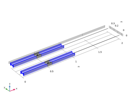
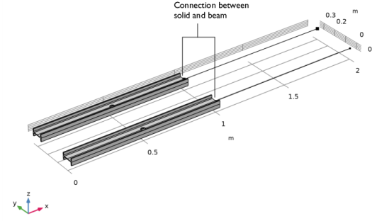
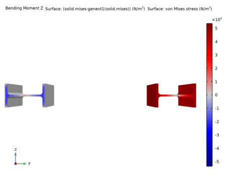
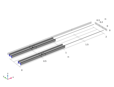
Length of each beam: 2 m. The transition is at the midpoint.
Cross section of the beam: European standard I-section beam (IPE 80) of 80-by-46 mm with 3.8 mm web thickness and 5.2 mm flange thickness.
Material
The material is Structural Steel with the following data:
Young’s modulus, E = 200 GPa.
Constraints
The inner end of the solid modeled beam is fixed.
Load
In order to compare the behavior of structure under various loading conditions, six different load cases are analyzed separately. A unit point load (as force or moment) is applied at the free end of the beam in three different directions.
Results and Discussion
The von Mises stress distribution for the load case with moment about the X-axis (the “twisting moment” load case) is plotted and compared for both connection types. As shown in Figure 2, the stress distribution seems to be comparable for both cases except near the solid-beam connections.
Figure 2: The von Mises stress distribution of the Twisting Moment load case.
To compare the behavior of both connection types, the von Mises stress distribution for the load case with moment about the Z axis (the “bending moment Z” load case) is plotted, along with the difference in von Mises distribution between the two. As can be seen in Figure 3, the stress distribution is comparable throughout the structure except near the solid-beam interface.
Figure 3: Comparison of von Mises stress distribution under Bending Moment Z load case.
To compare the performance of the two connection types, the traction distribution at the solid-beam interface for different load cases are plotted as shown in Figure 4 and Figure 5. For the load case with twisting moment, the transition connection type shows an in-plane distribution of traction, while the traction in the second case is predominantly out of plane. Similarly, for the load case with moment about the Z-axis, a uniform distribution of traction across the cross section is observed for the first type compared to the general connection type in the second case.
Figure 4: Traction distribution at the solid-beam interface for the twisting moment load case.
Figure 5: Traction distribution at solid-beam interface for bending moment Z load case.
Notes About the COMSOL Implementation
The built-in multiphysics coupling Solid-Beam Connection is used to connect the Solid and Beam interfaces in this model. The connection type Solid boundaries to beam points, transition includes warping of the cross section. The variables of warping are separately solved for in a stationary step, by clearing the selection of all other physics interfaces except the Solid-Beam Connection multiphysics coupling. In the subsequent study steps, these variables are manually suppressed to solve for the other variables of the study. If warping is insignificant for a certain connection, then you can select to ignore it, thus simplifying the solver setup.
Application Library path: Structural_Mechanics_Module/Beams_and_Shells/beam_solid_connection
Modeling Instructions
From the File menu, choose New.
New
In the New window, click  Model Wizard.
Model Wizard
1
In the Model Wizard window, click  3D.
2
In the Select Physics tree, select Structural Mechanics>Solid Mechanics (solid).
3
Click Add.
4
In the Select Physics tree, select Structural Mechanics>Beam (beam).
5
Click Add.
6
Click  Study.
7
In the Select Study tree, select General Studies>Stationary.
8
Global Definitions
Parameters 1
1
In the Model Builder window, under Global Definitions click Parameters 1.
2
In the Settings window for Parameters, locate the Parameters section.
3
Click  Load from File.
4
Load Group Mx
1
In the Model Builder window, right-click Global Definitions and choose Load and Constraint Groups>Load Group.
2
In the Settings window for Load Group, type Load Group Mx in the Label text field.
3
In the Parameter name text field, type lgMx.
Load Group My
1
In the Model Builder window, right-click Load and Constraint Groups and choose Load Group.
2
In the Settings window for Load Group, type Load Group My in the Label text field.
3
In the Parameter name text field, type lgMy.
Load Group Mz
1
Right-click Load and Constraint Groups and choose Load Group.
2
In the Settings window for Load Group, type Load Group Mz in the Label text field.
3
In the Parameter name text field, type lgMz.
Load Group Fx
1
Right-click Load and Constraint Groups and choose Load Group.
2
In the Settings window for Load Group, type Load Group Fx in the Label text field.
3
In the Parameter name text field, type lgFx.
Load Group Fy
1
Right-click Load and Constraint Groups and choose Load Group.
2
In the Settings window for Load Group, type Load Group Fy in the Label text field.
3
In the Parameter name text field, type lgFy.
Load Group Fz
1
Right-click Load and Constraint Groups and choose Load Group.
2
In the Settings window for Load Group, type Load Group Fz in the Label text field.
3
In the Parameter name text field, type lgFz.
The following section provides step by step instructions to create the geometry from scratch. If you do not want to build the geometry yourself, you can load the geometry sequence from the stored model. In the Model Builder window, under Component 1 (comp1) right-click Geometry 1 and choose Insert Sequence. Browse to the model’s Application Libraries folder and double-click the file beam_solid_connection.mph.
You can then skip the section about creating Geometry 1 and continue to the Definitions section.
Geometry 1
Polygon 1 (pol1)
1
In the Geometry toolbar, click  More Primitives and choose Polygon.
2
In the Settings window for Polygon, locate the Coordinates section.
3
From the Data source list, choose Vectors.
4
In the x text field, type L 2*L.
5
In the y text field, type 0 0.
6
In the z text field, type 0 0.
7
Click  Build Selected.
8
Click the  Zoom Extents button in the Graphics toolbar.
Work Plane 1 (wp1)
1
In the Geometry toolbar, click  Work Plane.
2
In the Settings window for Work Plane, locate the Plane Definition section.
3
From the Plane list, choose zy-plane.
4
Click  Build Selected.
Work Plane 1 (wp1)>Plane Geometry
In the Model Builder window, click Plane Geometry.
Part Libraries
1
In the Home toolbar, click  Windows and choose Part Libraries.
2
In the Part Libraries window, select Structural Mechanics Module>Beams>European Standard>IPE_beam in the tree.
3
Click  Add to Geometry.
Geometry 1
Work Plane 1 (wp1)>European IPE-beam 1 (pi1)
1
In the Model Builder window, under Component 1 (comp1)>Geometry 1>Work Plane 1 (wp1)>Plane Geometry click European IPE-beam 1 (pi1).
2
In the Settings window for Part Instance, click  Build Selected.
Extrude 1 (ext1)
1
In the Model Builder window, right-click Geometry 1 and choose Extrude.
2
In the Settings window for Extrude, locate the Distances section.
3
4
Select the Reverse direction check box.
5
Click  Build Selected.
Cylinder 1 (cyl1)
1
In the Geometry toolbar, click  Cylinder.
2
In the Settings window for Cylinder, locate the Size and Shape section.
3
In the Radius text field, type R.
4
In the Height text field, type L.
5
Locate the Position section. In the x text field, type L/2.
6
In the z text field, type -L/2.
7
Click  Build Selected.
Difference 1 (dif1)
1
In the Geometry toolbar, click  Booleans and Partitions and choose Difference.
2
3
In the Settings window for Difference, locate the Difference section.
4
Find the Objects to subtract subsection. Select the  Activate Selection toggle button.
5
6
Click  Build Selected.
Copy 1 (copy1)
1
In the Geometry toolbar, click  Transforms and choose Copy.
2
Click in the Graphics window and then press Ctrl+A to select both objects.
3
In the Settings window for Copy, locate the Displacement section.
4
In the y text field, type 0.3*L.
5
Click  Build Selected.
6
Click the  Zoom Extents button in the Graphics toolbar.
Work Plane 2 (wp2)
1
In the Geometry toolbar, click  Work Plane.
2
In the Settings window for Work Plane, locate the Plane Definition section.
3
From the Plane list, choose zy-plane.
4
In the x-coordinate text field, type 0.45*L.
5
Click  Build Selected.
Work Plane 3 (wp3)
1
Right-click Work Plane 2 (wp2) and choose Duplicate.
2
In the Settings window for Work Plane, locate the Plane Definition section.
3
In the x-coordinate text field, type 0.55*L.
4
Click  Build Selected.
Partition Objects 1 (par1)
1
In the Geometry toolbar, click  Booleans and Partitions and choose Partition Objects.
2
Select the objects copy1(1) and dif1 only.
3
In the Settings window for Partition Objects, locate the Partition Objects section.
4
From the Partition with list, choose Work plane.
5
From the Work plane list, choose Work Plane 2 (wp2).
6
Click  Build Selected.
Partition Objects 2 (par2)
1
Right-click Partition Objects 1 (par1) and choose Duplicate.
2
Select the objects par1(1) and par1(2) only.
3
In the Settings window for Partition Objects, locate the Partition Objects section.
4
From the Work plane list, choose Work Plane 3 (wp3).
5
Click  Build Selected.
Union 1 (uni1)
1
In the Geometry toolbar, click  Booleans and Partitions and choose Union.
2
Select the object par2(2) only.
3
In the Settings window for Union, click  Build Selected.
Union 2 (uni2)
1
In the Geometry toolbar, click  Booleans and Partitions and choose Union.
2
Select the object par2(1) only.
3
In the Settings window for Union, click  Build Selected.
Form Union (fin)
1
In the Model Builder window, under Component 1 (comp1)>Geometry 1 click Form Union (fin).
2
In the Settings window for Form Union/Assembly, locate the Form Union/Assembly section.
3
From the Action list, choose Form an assembly.
4
In the Geometry toolbar, click  Build All.
Fixed End
1
In the Geometry toolbar, click  Selections and choose Explicit Selection.
2
In the Settings window for Explicit Selection, type Fixed End in the Label text field.
3
Locate the Entities to Select section. From the Geometric entity level list, choose Boundary.
4
On the object fin, select Boundaries 1 and 69 only.
It might be easier to select the boundaries by using the Selection List window. To open this window, in the Home toolbar click Windows and choose Selection List. (If you are running the cross-platform desktop, you find Windows in the main menu.)
Solid Beam Interface
1
In the Geometry toolbar, click  Selections and choose Explicit Selection.
2
In the Settings window for Explicit Selection, type Solid Beam Interface in the Label text field.
3
Locate the Entities to Select section. From the Geometric entity level list, choose Boundary.
4
On the object fin, select Boundaries 68 and 136 only.
Free End
1
In the Geometry toolbar, click  Selections and choose Explicit Selection.
2
In the Settings window for Explicit Selection, type Free End in the Label text field.
3
Locate the Entities to Select section. From the Geometric entity level list, choose Point.
4
On the object fin, select Points 178 and 180 only.
Definitions
General Extrusion 1 (genext1)
1
In the Definitions toolbar, click  Nonlocal Couplings and choose General Extrusion.
2
3
In the Settings window for General Extrusion, locate the Destination Map section.
4
In the x-expression text field, type X.
5
In the y-expression text field, type Y+0.3*L.
6
In the z-expression text field, type Z.
7
Locate the Source section. From the Source frame list, choose Material  (X, Y, Z).
Add Material
Structural steel is used for all the components of the structure, and thus it can be added as a Global Material in the model. Using the Material Link node, you can assign the Global Material to different domains, boundaries, and edges of the structure.
1
In the Home toolbar, click  Add Material to open the Add Material window.
2
Go to the Add Material window.
3
In the tree, select Built-in>Structural steel.
4
Click the right end of the Add to Component split button in the window toolbar.
5
From the menu, choose Add to Global Materials.
6
In the Home toolbar, click  Add Material to close the Add Material window.
Materials
Material Link 1 (matlnk1)
In the Model Builder window, under Component 1 (comp1) right-click Materials and choose More Materials>Material Link.
Material Link 2 (matlnk2)
1
Right-click Materials and choose More Materials>Material Link.
2
In the Settings window for Material Link, locate the Geometric Entity Selection section.
3
From the Geometric entity level list, choose Edge.
4
Add physics settings for the Solid Mechanics interface.
Solid Mechanics (solid)
1
In the Model Builder window, under Component 1 (comp1) click Solid Mechanics (solid).
2
In the Settings window for Solid Mechanics, click to expand the Discretization section.
3
From the Displacement field list, choose Linear.
Fixed Constraint 1
1
In the Physics toolbar, click  Boundaries and choose Fixed Constraint.
2
In the Settings window for Fixed Constraint, locate the Boundary Selection section.
3
From the Selection list, choose Fixed End.
Add physics settings for the Beam interface.
Beam (beam)
1
In the Model Builder window, under Component 1 (comp1) click Beam (beam).
2
In the Settings window for Beam, locate the Edge Selection section.
3
Click  Clear Selection.
4
Cross-Section Data 1
1
In the Model Builder window, under Component 1 (comp1)>Beam (beam) click Cross-Section Data 1.
2
In the Settings window for Cross-Section Data, locate the Basic Section Properties section.
3
In the A text field, type A.
4
In the Izz text field, type Izz.
5
In the ez text field, type ez.
6
In the Iyy text field, type Iyy.
7
In the ey text field, type ey.
8
In the J text field, type J.
9
Click to expand the Stress Evaluation Properties section. In the hy text field, type hy.
10
In the hz text field, type hz.
11
In the wt text field, type Wt.
12
In the μy text field, type muy.
13
In the μz text field, type muz.
Section Orientation 1
1
In the Model Builder window, click Section Orientation 1.
2
In the Settings window for Section Orientation, locate the Section Orientation section.
3
From the Orientation method list, choose Orientation vector.
4
Specify the V vector as
Point Load 1
1
In the Physics toolbar, click  Points and choose Point Load.
2
In the Settings window for Point Load, locate the Point Selection section.
3
From the Selection list, choose Free End.
4
Locate the Moment section. Specify the MP vector as
5
In the Physics toolbar, click  Load Group and choose Gravity Load.
Point Load 2
1
In the Physics toolbar, click  Points and choose Point Load.
2
In the Settings window for Point Load, locate the Point Selection section.
3
From the Selection list, choose Free End.
4
Locate the Moment section. Specify the MP vector as
5
In the Physics toolbar, click  Load Group and choose Load Group 2.
Point Load 3
1
In the Physics toolbar, click  Points and choose Point Load.
2
In the Settings window for Point Load, locate the Point Selection section.
3
From the Selection list, choose Free End.
4
Locate the Moment section. Specify the MP vector as
5
In the Physics toolbar, click  Load Group and choose Load Group 3.
Point Load 4
1
In the Physics toolbar, click  Points and choose Point Load.
2
In the Settings window for Point Load, locate the Point Selection section.
3
From the Selection list, choose Free End.
4
Locate the Force section. Specify the FP vector as
5
In the Physics toolbar, click  Load Group and choose Load Group 4.
Point Load 5
1
In the Physics toolbar, click  Points and choose Point Load.
2
In the Settings window for Point Load, locate the Point Selection section.
3
From the Selection list, choose Free End.
4
Locate the Force section. Specify the FP vector as
5
In the Physics toolbar, click  Load Group and choose Load Group 5.
Point Load 6
1
In the Physics toolbar, click  Points and choose Point Load.
2
In the Settings window for Point Load, locate the Point Selection section.
3
From the Selection list, choose Free End.
4
Locate the Force section. Specify the FP vector as
5
In the Physics toolbar, click  Load Group and choose Load Group 6.
Add couplings between the solid and the beam elements.
Multiphysics
Solid-Beam Connection Transition
1
In the Physics toolbar, click  Multiphysics Couplings and choose Global>Solid-Beam Connection.
2
In the Settings window for Solid-Beam Connection, type Solid-Beam Connection Transition in the Label text field.
3
Locate the Connection Settings section. From the Connection type list, choose Solid boundaries to beam points, transition.
4
Select the Manual control of selections check box.
5
Locate the Boundary Selection, Solid section. Select the  Activate Selection toggle button.
6
7
Locate the Point Selection, Beam section. Select the  Activate Selection toggle button.
8
Solid-Beam Connection General
1
In the Physics toolbar, click  Multiphysics Couplings and choose Global>Solid-Beam Connection.
2
In the Settings window for Solid-Beam Connection, type Solid-Beam Connection General in the Label text field.
3
Locate the Connection Settings section. Select the Manual control of selections check box.
4
5
Locate the Point Selection, Beam section. Select the  Activate Selection toggle button.
6
Mesh 1
Free Triangular 1
1
In the Mesh toolbar, click  Boundary and choose Free Triangular.
2
Size 1
1
Right-click Free Triangular 1 and choose Size.
2
In the Settings window for Size, locate the Element Size section.
3
Click the Custom button.
4
Locate the Element Size Parameters section. Select the Maximum element size check box.
5
6
Click  Build Selected.
Swept 1
1
In the Mesh toolbar, click  Swept.
2
In the Settings window for Swept, locate the Domain Selection section.
3
From the Geometric entity level list, choose Domain.
4
Distribution 1
1
Right-click Swept 1 and choose Distribution.
2
In the Settings window for Distribution, locate the Domain Selection section.
3
4
Click  Remove from Selection.
5
6
Locate the Distribution section. From the Distribution type list, choose Explicit.
7
In the Relative placement of vertices along edge text field, type range(0,0.015,1).
8
Click  Build Selected.
Distribution 2
1
In the Model Builder window, right-click Swept 1 and choose Distribution.
2
In the Settings window for Distribution, locate the Domain Selection section.
3
4
Click  Remove from Selection.
5
6
Locate the Distribution section. From the Distribution type list, choose Explicit.
7
In the Relative placement of vertices along edge text field, type range(0,0.015,0.92) range(0.92,0.005,1).
8
Select the Reverse direction check box.
9
Click  Build Selected.
Free Tetrahedral 1
1
In the Mesh toolbar, click  Free Tetrahedral.
2
In the Settings window for Free Tetrahedral, locate the Domain Selection section.
3
From the Geometric entity level list, choose Domain.
4
Size 1
1
Right-click Free Tetrahedral 1 and choose Size.
2
In the Settings window for Size, locate the Element Size section.
3
Click the Custom button.
4
Locate the Element Size Parameters section. Select the Maximum element size check box.
5
6
Click  Build Selected.
Edge 1
1
In the Mesh toolbar, click  Boundary and choose Edge.
2
Distribution 1
1
Right-click Edge 1 and choose Distribution.
2
In the Settings window for Distribution, locate the Distribution section.
3
In the Number of elements text field, type 10.
4
Click  Build All.
Study 1
Step 1: Stationary
1
In the Model Builder window, under Study 1 click Step 1: Stationary.
2
In the Settings window for Stationary, locate the Physics and Variables Selection section.
3
4
Click to expand the Values of Dependent Variables section. Find the Initial values of variables solved for subsection. From the Settings list, choose User controlled.
Stationary 2
1
In the Study toolbar, click  Study Steps and choose Stationary>Stationary.
2
In the Settings window for Stationary, click to expand the Study Extensions section.
3
Select the Define load cases check box.
4
Click  Add six times.
5
Solution 1 (sol1)
1
In the Study toolbar, click  Show Default Solver.
2
In the Model Builder window, expand the Solution 1 (sol1) node, then click Dependent Variables 1.
3
In the Settings window for Dependent Variables, locate the General section.
4
From the Defined by study step list, choose User defined.
5
In the Model Builder window, expand the Study 1>Solver Configurations>Solution 1 (sol1)>Dependent Variables 1 node, then click Displacement field (comp1.u).
6
In the Settings window for Field, locate the General section.
7
Clear the Solve for this field check box.
8
In the Model Builder window, click Dependent Variables 2.
9
In the Settings window for Dependent Variables, locate the General section.
10
From the Defined by study step list, choose User defined.
11
In the Model Builder window, expand the Study 1>Solver Configurations>Solution 1 (sol1)>Dependent Variables 2 node, then click Displacement field (comp1.u).
12
In the Settings window for Field, locate the Scaling section.
13
From the Method list, choose Manual.
14
In the Scale text field, type 1.0e-10.
15
In the Model Builder window, click Displacement field (comp1.u2).
16
In the Settings window for Field, locate the Scaling section.
17
From the Method list, choose Manual.
18
In the Scale text field, type 1.0e-10.
19
In the Model Builder window, click Warping function (comp1.sbc1.ww).
20
In the Settings window for Field, locate the General section.
21
Clear the Solve for this field check box.
22
In the Model Builder window, click Warping constant (comp1.sbc1.C0).
23
In the Settings window for State, locate the General section.
24
Clear the Solve for this state check box.
25
In the Model Builder window, click Warping constant (comp1.sbc1.C1).
26
In the Settings window for State, locate the General section.
27
Clear the Solve for this state check box.
28
In the Model Builder window, click Warping constant (comp1.sbc1.C2).
29
In the Settings window for State, locate the General section.
30
Clear the Solve for this state check box.
31
In the Study toolbar, click  Compute.
Definitions
View 1
1
In the Model Builder window, under Component 1 (comp1)>Definitions click View 1.
2
In the Settings window for View, locate the View section.
3
Clear the Show grid check box.
Use the following instructions to plot the von Mises stress distribution shown in Figure 2.
Results
Stress (solid)
1
In the Model Builder window, under Results click Stress (solid).
2
In the Settings window for 3D Plot Group, locate the Data section.
3
From the Load case list, choose Twisting Moment.
4
Locate the Plot Settings section. Clear the Plot dataset edges check box.
Line 1
1
In the Model Builder window, expand the Stress (beam) node.
2
Right-click Line 1 and choose Copy.
Line 1
1
In the Model Builder window, right-click Stress (solid) and choose Paste Line.
2
In the Settings window for Line, locate the Expression section.
3
In the Expression text field, type if(group.lgMx,beam.ttmax*sqrt(3),beam.mises).
4
Click to expand the Inherit Style section. From the Plot list, choose Surface 1.
5
In the Stress (solid) toolbar, click  Plot.
6
Click the  Zoom Extents button in the Graphics toolbar.
Use the following instructions to plot the comparison of von Mises stress distribution shown in Figure 3.
Comparison
1
In the Home toolbar, click  Add Plot Group and choose 3D Plot Group.
2
In the Settings window for 3D Plot Group, type Comparison in the Label text field.
3
Locate the Data section. From the Load case list, choose Bending Moment Z.
4
Locate the Plot Settings section. Clear the Plot dataset edges check box.
Surface 1
1
Right-click Comparison and choose Surface.
2
In the Settings window for Surface, locate the Expression section.
3
In the Expression text field, type (solid.mises-genext1(solid.mises)).
4
Locate the Coloring and Style section. From the Color table list, choose Wave.
5
Select the Symmetrize color range check box.
Surface 2
1
In the Model Builder window, right-click Comparison and choose Surface.
2
In the Settings window for Surface, locate the Expression section.
3
In the Expression text field, type solid.mises.
4
Click to expand the Inherit Style section. From the Plot list, choose Surface 1.
Selection 1
1
Right-click Surface 2 and choose Selection.
2
3
In the Comparison toolbar, click  Plot.
To see the stress distribution at the solid-beam interface, select the YZ View.
4
Click the  Go to YZ View button in the Graphics toolbar.
For different load cases, the traction at the solid-beam interface is compared for both Solid-Beam Connection types as shown in Figure 4 and Figure 5.
Study 1/Solution 1 (3) (sol1)
In the Results toolbar, click  More Datasets and choose Solution.
Selection
1
In the Results toolbar, click  Attributes and choose Selection.
2
In the Settings window for Selection, locate the Geometric Entity Selection section.
3
From the Geometric entity level list, choose Boundary.
4
From the Selection list, choose Solid Beam Interface.
Traction
1
In the Results toolbar, click  3D Plot Group.
2
In the Settings window for 3D Plot Group, type Traction in the Label text field.
3
Locate the Data section. From the Dataset list, choose Study 1/Solution 1 (3) (sol1).
4
From the Load case list, choose Twisting Moment.
5
Locate the Plot Settings section. Clear the Plot dataset edges check box.
Surface 1
1
Right-click Traction and choose Surface.
2
In the Settings window for Surface, locate the Expression section.
3
In the Expression text field, type solid.mises.
Arrow Surface 1
1
In the Model Builder window, right-click Traction and choose Arrow Surface.
2
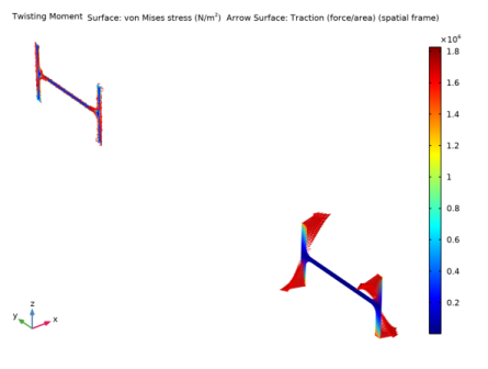
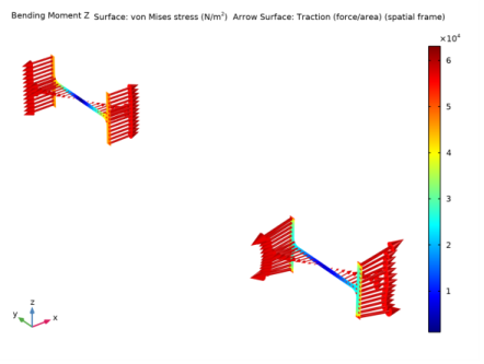
In the Settings window for Arrow Surface, click Replace Expression in the upper-right corner of the Expression section. From the menu, choose Component 1 (comp1)>Solid Mechanics>Stress>solid.Tax,...,solid.Taz - Traction (force/area) (spatial frame).
3
Locate the Arrow Positioning section. In the Number of arrows text field, type 1000.
4
Click to expand the Inherit Style section. From the Plot list, choose Surface 1.
5
In the Traction toolbar, click  Plot.
6
Click the  Zoom Extents button in the Graphics toolbar.
Traction
1
In the Model Builder window, click Traction.
2
In the Settings window for 3D Plot Group, locate the Data section.
3
From the Load case list, choose Bending Moment Z.
Arrow Surface 1
1
In the Model Builder window, click Arrow Surface 1.
2
In the Settings window for Arrow Surface, locate the Arrow Positioning section.
3
In the Number of arrows text field, type 120.
4
In the Traction toolbar, click  Plot.