You are viewing the documentation for an older COMSOL version. The latest version is available here.
PDF

Step Thrust Bearing
Introduction
In this example the pressure distribution in a step thrust bearing is analyzed. A step thrust bearing consists of a stepped bearing surface on which the end of the shaft rotates. The entire assembly is submerged in a lubricant. A six step thrust bearing is considered in this example. The shaft collar is assumed to be spinning without any axial motion in the bearing. The simulation is performed using the Rotordynamics Module’s Hydrodynamic Bearing interface. This interface solves the Reynolds equation to compute the pressure developed in a thin fluid film.
Model Definition
A six pad step thrust bearing is considered. Pad inner and outer diameters are 0.1 m and 0.2 m, respectively. Groove angle between the pads is 15° and its depth is 0.0001 m relative to the pad surface. Clearance between the pad and the collar surface is 0.0001 m.
The shaft is spinning with an angular speed Ω (1000 rad/s). However, It is not moving in axial direction. So the film thickness does not change due to the shaft motion.
The bearing geometry is shown in Figure 1 below.
Figure 1: Step thrust bearing geometry.
Effect of the cavitation is also included to compute the pressure distribution in the fluid film. Following fluid properties are needed — the dynamic viscosity, the density at cavitation pressure, and the compressibility. The fluid parameters, whose values are summarized in Table 1, are close to those of lubricating oils used in real bearings.
10-7 Pa-1
Results and Discussion
Figure 2 below shows the fluid pressure profile on the bearing.
Figure 2: Fluid film pressure profile.
For the above pressure distribution, the total vertical force on the collar is 15,488 N. This is the load carrying capacity of the bearing at the specified speed.
Mass fraction of the lubricant which is a measure of the cavitation is shown in Figure 3. From the figure it is clear that amount of cavitation is very small and is localized near the trailing edge of the pad.
Figure 3: Mass fraction.
The pressure distribution on the pad in radial and circumferential directions are shown in Figure 4 and Figure 5. Pressure at the inner and outer radius locations are zero with the distribution marginally biased toward the outer side. The velocity of the collar varies linearly from inner radius to outer radius. Since the pressure distribution is proportional to the shear velocity in the film, it should have increased linearly from inner point to the outer point. However, at the ends the film pressure is set to zero. Therefore, maximum pressure occurs toward the outer side from the mid position. In the circumferential direction the pressure suddenly rises at the step location (leading edge of the pad) and drops down slowly toward the trailing edge.
Figure 4: Pressure profile in radial direction.
Figure 5: Pressure profile in circumferential direction.
Figure 6 shows bearing profile computed using the film thickness.
Figure 6: Bearing profile.
Application Library path: Rotordynamics_Module/Tutorials/step_thrust_bearing
Modeling Instructions
From the File menu, choose New.
New
In the New window, click  Model Wizard.
Model Wizard
1
In the Model Wizard window, click  3D.
2
In the Select Physics tree, select Structural Mechanics>Rotordynamics>Hydrodynamic Bearing (hdb).
3
Click Add.
4
Click  Study.
5
In the Select Study tree, select General Studies>Stationary.
6
Global Definitions
Parameters 1
1
In the Model Builder window, under Global Definitions click Parameters 1.
2
In the Settings window for Parameters, locate the Parameters section.
3
Geometry 1
Work Plane 1 (wp1)
In the Geometry toolbar, click  Work Plane.
Work Plane 1 (wp1)>Plane Geometry
In the Model Builder window, click Plane Geometry.
Work Plane 1 (wp1)>Circle 1 (c1)
1
In the Work Plane toolbar, click  Circle.
2
In the Settings window for Circle, locate the Size and Shape section.
3
In the Radius text field, type Ro.
4
In the Sector angle text field, type gAng.
5
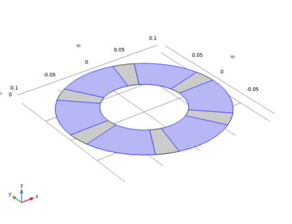
Click to expand the Layers section. In the table, enter the following settings:
Work Plane 1 (wp1)>Circle 2 (c2)
1
Right-click Component 1 (comp1)>Geometry 1>Work Plane 1 (wp1)>Plane Geometry>Circle 1 (c1) and choose Duplicate.
2
In the Settings window for Circle, locate the Size and Shape section.
3
In the Sector angle text field, type 360/N-gAng.
4
Locate the Rotation Angle section. In the Rotation text field, type gAng.
Delete Entities 1 (del1)
1
In the Model Builder window, right-click Geometry 1 and choose Delete Entities.
2
On the object wp1, select Boundaries 1 and 2 only.
Rotate 1 (rot1)
1
In the Geometry toolbar, click  Transforms and choose Rotate.
2
3
In the Settings window for Rotate, locate the Rotation section.
4
In the Angle text field, type range(0,360/N,360-360/N).
5
Click  Build All Objects.
6
Click the  Zoom Extents button in the Graphics toolbar.
In the step bearing, the film thickness varies in steps with one value in the groove and another on the pad. Define a film thickness variable hf in two separate Variable nodes with complementary selections to specify different values in different regions.
Definitions
Variables 1
1
In the Model Builder window, under Component 1 (comp1) right-click Definitions and choose Variables.
2
In the Settings window for Variables, locate the Variables section.
3
4
Locate the Geometric Entity Selection section. From the Geometric entity level list, choose Boundary.
5
It might be easier to select the correct boundaries by using the Selection List window. To open this window, in the Home toolbar click Windows and choose Selection List. (If you are running the cross-platform desktop, you find Windows in the main menu.)
Variables 2
1
Right-click Variables 1 and choose Duplicate.
2
In the Settings window for Variables, locate the Variables section.
3
4
Locate the Geometric Entity Selection section. Click  Clear Selection.
5
Hydrodynamic Bearing (hdb)
1
Click the  Show More Options button in the Model Builder toolbar.
2
In the Show More Options dialog box, in the tree, select the check box for the node Physics>Advanced Physics Options.
3
Enable the Cavitation formulation in the bearing.
4
In the Model Builder window, under Component 1 (comp1) click Hydrodynamic Bearing (hdb).
5
In the Settings window for Hydrodynamic Bearing, click to expand the Cavitation section.
6
Select the Cavitation check box.
Reduce the Cavitation transition width for the sharper transition between the cavitated and non cavitated regions.
7
In the Δpsw text field, type 0.5[MPa].
Change the Stabilization tuning parameter for better stabilization in the cavitated region.
8
Click the  Show More Options button in the Model Builder toolbar.
9
In the Show More Options dialog box, in the tree, select the check box for the node Physics>Stabilization.
10
11
In the Settings window for Hydrodynamic Bearing, click to expand the Inconsistent Stabilization section.
12
In the δartificial text field, type 50.
Hydrodynamic Thrust Bearing 1
1
In the Physics toolbar, click  Boundaries and choose Hydrodynamic Thrust Bearing.
Because the reference surface is assumed to be located on the collar, change the Reference normal orientation to align it with the collar normal.
2
In the Settings window for Hydrodynamic Thrust Bearing, locate the Reference Surface Properties section.
3
From the Reference normal orientation list, choose Opposite direction to geometry normal.
4
Locate the Bearing Properties section. From the Bearing type list, choose User defined.
5
In the hb1 text field, type hf.
6
Locate the Collar Properties section. In the Ω text field, type 1000.
7
Locate the Fluid Properties section. From the μ list, choose User defined. In the associated text field, type 0.072[Pa*s].
8
In the ρc text field, type 866[kg/m^3].
9
Click in the Graphics window and then press Ctrl+A to select all boundaries.
Bearing Orientation 1
1
In the Model Builder window, click Bearing Orientation 1.
2
In the Settings window for Bearing Orientation, locate the Bearing Orientation section.
3
From the Axis list, choose z-axis.
4
Specify the Orientation vector defining local y direction vector as
Mesh 1
Mapped 1
1
In the Mesh toolbar, click  Boundary and choose Mapped.
2
In the Settings window for Mapped, locate the Boundary Selection section.
3
From the Selection list, choose All boundaries.
Create one element per degree in the azimuthal direction to capture the pressure accurately.
Distribution 1
1
Right-click Mapped 1 and choose Distribution.
2
3
In the Settings window for Distribution, locate the Distribution section.
4
In the Number of elements text field, type 360/N-gAng.
Distribution 2
1
In the Model Builder window, right-click Mapped 1 and choose Distribution.
2
3
In the Settings window for Distribution, locate the Distribution section.
4
In the Number of elements text field, type gAng.
Distribution 3
1
Right-click Mapped 1 and choose Distribution.
2
3
In the Settings window for Distribution, locate the Distribution section.
4
In the Number of elements text field, type 20.
5
Click  Build All.
Study 1
In the Home toolbar, click  Compute.
Results
Default plot shows the pressure distribution in the bearing. To generate the height plot for the pressure distribution shown in Figure 2 start by creating a Surface dataset.
Surface 1
1
In the Results toolbar, click  More Datasets and choose Surface.
2
In the Settings window for Surface, locate the Selection section.
3
From the Selection list, choose All boundaries.
Pressure (Height)
1
In the Results toolbar, click  2D Plot Group.
2
In the Settings window for 2D Plot Group, type Pressure (Height) in the Label text field.
Surface 1
1
Right-click Pressure (Height) and choose Surface.
2
In the Settings window for Surface, locate the Expression section.
3
In the Expression text field, type hdb.p.
4
Locate the Coloring and Style section. From the Color table list, choose Traffic.
Height Expression 1
1
Right-click Surface 1 and choose Height Expression.
2
In the Settings window for Height Expression, locate the Axis section.
3
Select the Scale factor check box.
4
5
Click the  Go to Default View button in the Graphics toolbar.
6
In the Pressure (Height) toolbar, click  Plot.
Evaluate the load on the collar.
Global Evaluation 1
1
In the Results toolbar, click  Global Evaluation.
2
In the Settings window for Global Evaluation, click Replace Expression in the upper-right corner of the Expressions section. From the menu, choose Component 1 (comp1)>Hydrodynamic Bearing>Fluid loads>Fluid load on collar - N>hdb.htb1.Fcz - Fluid load on collar, z component.
3
Click  Evaluate.
The following instructions are to plot the mass fraction of the lubricant shown in Figure 3.
Mass Fraction
1
In the Results toolbar, click  3D Plot Group.
2
In the Settings window for 3D Plot Group, type Mass Fraction in the Label text field.
Contour 1
1
Right-click Mass Fraction and choose Contour.
2
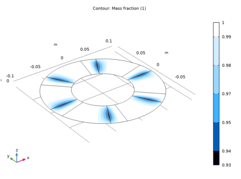
In the Settings window for Contour, click Replace Expression in the upper-right corner of the Expression section. From the menu, choose Component 1 (comp1)>Hydrodynamic Bearing>Cavitation>hdb.theta - Mass fraction.
3
Locate the Coloring and Style section. From the Contour type list, choose Filled.
4
Locate the Levels section. In the Total levels text field, type 5.
5
Locate the Coloring and Style section. From the Color table list, choose JupiterAuroraBorealis.
6
Click the  Go to Default View button in the Graphics toolbar.
7
In the Mass Fraction toolbar, click  Plot.
Figure 6 shows the bearing profile. Follow the instructions below to replicate it.
2D Plot Group 4
In the Home toolbar, click  Add Plot Group and choose 2D Plot Group.
Surface 1
1
Right-click 2D Plot Group 4 and choose Surface.
2
In the Settings window for Surface, locate the Expression section.
3
In the Expression text field, type hg-hdb.h.
4
Locate the Coloring and Style section. From the Coloring list, choose Uniform.
5
From the Color list, choose Gray.
Height Expression 1
1
Right-click Surface 1 and choose Height Expression.
2
In the Settings window for Height Expression, locate the Axis section.
3
Select the Scale factor check box.
4
Pad Profile
1
In the Model Builder window, under Results click 2D Plot Group 4.
2
In the Settings window for 2D Plot Group, type Pad Profile in the Label text field.
3
Locate the Plot Settings section. Clear the Plot dataset edges check box.
4
Click the  Go to Default View button in the Graphics toolbar.
5
In the Pad Profile toolbar, click  Plot.
You can also analyze the pressure distributions along the radial and circumferential directions of the bearing shown in Figure 4 and Figure 5. Start by creating a Cut line along the radial line.
Cut Line 3D: Radial line
1
In the Results toolbar, click  Cut Line 3D.
2
In the Settings window for Cut Line 3D, locate the Line Data section.
3
In row Point 2, set X to 0.
4
In row Point 2, set Y to Ro.
5
6
In the Label text field, type Cut Line 3D: Radial line.
Pressure (Radial distribution)
1
In the Results toolbar, click  1D Plot Group.
2
In the Settings window for 1D Plot Group, type Pressure (Radial distribution) in the Label text field.
3
Locate the Data section. From the Dataset list, choose Cut Line 3D: Radial line.
Line Graph 1
1
Right-click Pressure (Radial distribution) and choose Line Graph.
2
In the Settings window for Line Graph, locate the y-Axis Data section.
3
In the Expression text field, type hdb.p.
4
In the Pressure (Radial distribution) toolbar, click  Plot.
Use the Parameterized Curve to create the circumferential sector line.
Parameterized Curve 3D: Circumferential line
1
In the Results toolbar, click  More Datasets and choose Parameterized Curve 3D.
2
In the Settings window for Parameterized Curve 3D, locate the Parameter section.
3
In the Maximum text field, type 2*pi/N.
4
Locate the Expressions section. In the x text field, type 0.5*(Ro+Ri)*cos(s).
5
In the y text field, type 0.5*(Ro+Ri)*sin(s).
6
In the Label text field, type Parameterized Curve 3D: Circumferential line.
7
Pressure (Circumferential distribution)
1
In the Model Builder window, right-click Pressure (Radial distribution) and choose Duplicate.
2
In the Settings window for 1D Plot Group, locate the Data section.
3
From the Dataset list, choose Parameterized Curve 3D: Circumferential line.
4
In the Label text field, type Pressure (Circumferential distribution).
5
In the Pressure (Circumferential distribution) toolbar, click  Plot.