Compact Camera Module

Compact camera modules are widely used in electronic devices such as mobile phones and tablet computers. In order to reduce both the size and number of elements required the optical design will typically incorporate several highly aspheric surfaces. This model demonstrates a five element (plus filter) design using the 'Aspheric Even Lens 3D' part from the Ray Optics Module part library.

Model Definition

An overview of the optical design of the compact camera module used in this tutorial is shown in Figure 1. The prescription for this lens design can be found in Ref. 1. It has a 7.0 mm focal length, a f/2.4 focal ratio, and a nominal field of view of 36°.

Figure 1: Overview of the Compact Camera Module optical design. In this cross-section view, the rays have been colored by release index.

The detailed optical prescription is given in Table 1. Instructions for creating the lens geometry sequence (Figure 2) can be found in the Appendix — Geometry Instructions. In addition to the parameters used to define the Compact Camera Module geometry, a set of parameters are required to define the ray tracing model. These are listed in Table 2.

Table 1: Compact Camera Module Optical Prescription.
Index	Name	Radius (mm)	Conic constant	Thickness (mm)	Refractive index	Diameter (mm)
0	Object	∞	—	∞	—	—
1	Stop	∞	—	0.0000	—	2.50
2	Lens 1	1.679	0.22669364	1.1080	1.544	2.90
2	Lens 1	Aspheric coefficients:	A4 = 9.80281·10-3, A6 = -3.81227·10-2, A8 = 2.39681·10-2, A10 = -6.29128·10-3, A12 = -2.75496·10-3, A14 = -2.69638·10-4
3		-9.162	0	0.1000	—	3.05
3		Aspheric coefficients:	A4 = 3.73187·10-2, A6 = -8.91760·10-3, A8 = -5.89384·10-2, A10 = 4.41115·10-2, A12 = -1.26858·10-2, A14 = 1.16125·10-3
4	Lens 2	-15.649	0	0.2300	1.632	2.70
4	Lens 2	Aspheric coefficients:	A4 = 6.93172·10-2, A6 = -4.31157·10-2, A8 = 2.33346e·10-2, A10 = -2.33074·10-2, A12 = 2.22119·10-2, A14 = -4.84076·10-3
5		3.482	8.70133393	1.1305	—	2.21
5		Aspheric coefficients:	A4 = 5.21579·10-3, A6 = 7.15829·10-2, A8 = -4.60926·10-2, A10 = 1.24310·10-2, A12 = 3.32216e·10-2
6	Lens 3	-12.801	0	0.2300	1.632	2.30
6	Lens 3	Aspheric coefficients:	A4 = 3.96000·10-2, A6 = -3.42179·10-2, A8 = 7.75523·10-2, A10 = -4.22361·10-2
7		21.119	0	1.0559	—	2.25
7		Aspheric coefficients:	A4 = 1.01117·10-1, A6 = -3.21118·10-2, A8 = 9.03668·10-2, A10 = -3.37156·10-2, A12 = -6.52751·10-3
8	Lens 4	-3.266	0.85965815	0.2300	1.544	2.95
8	Lens 4	Aspheric coefficients:	A4 = -4.91398·10-2, A6 = -5.57533·10-3, A8 = 1.31557·10-2, A10 = 1.22280·10-3, A12 = -9.54019·10-4, A14 = -2.40349·10-6
9		2.724	0	0.1000	—	3.75
9		Aspheric coefficients:	A4 = -8.88955·10-2, A6 = 2.87927·10-2, A8 = -8.83436·10-3, A10 = 1.57329·10-3, A12 = -2.24134·10-4
10	Lens 5	5.272	0	1.0356	1.632	3.90
10	Lens 5	Aspheric coefficients:	A4 = -2.38313·10-2, A6 = 5.50321·10-3, A8 = -9.19080·10-4, A10 = -9.80631·10-5
11		-4.681	3.15790955	0.1337	—	4.00
11		Aspheric coefficients:	A4 = -3.17139·10-2, A6 = 3.80781·10-3, A8 = 3.43810·10-4, A10 = -3.27888·10-5
12	IR Filter	∞	0	0.2100	1.516	4.50
13		∞	0	0.1363	—	4.50
14	Image Plane	∞	0	—	—	5.00

Figure 2: The Compact Camera Module geometry sequence. Instructions for creating the lens geometry can be found in the Appendix.

Table 2: Compact Camera Module Model Definitions.
Parameter	Value	Description
λvac	587.56 nm	Vacuum wavelength
nref,1	1.544	Lens 1 and 4 refractive index (at 587.56 nm)
nref,2	1.632	Lens 2, 3, and 5 refractive index (at 587.56 nm)
nref,3	1.516	IR filter refractive index (at 587.56 nm)
Dpupil	2.50 mm	Entrance pupil diameter
Nring	25	Number of hexapolar rings. (Nrays = 1951)
θ1	0°	Field angle 1
θ2	5°	Field angle 2
θ3	10°	Field angle 3
θ4	15°	Field angle 4
Δz	-0.5 mm	Ray release z-coordinate

The ray tracing algorithm used by the Geometrical Optics interface computes the refracted ray direction based on a discretized geometry via the underlying finite element mesh. In this model, a cubic geometry shape order is used in order to reduce the discretization error. However, it is sometimes necessary to refine the mesh on certain surfaces in order to further reduce the effects of discretization. The aspheric surfaces of the Compact Camera Module have been assigned to a cumulative selection (Figure 3) on which the mesh has been refined (Figure 4).¹

The Compact Camera Module is assumed to be operating in air at room temperature. The wavelength is set to λ = 587.56 nm (that is, the wavelength at which the refractive indices are specified). Other Geometrical Optics features include the use of cumulative selections to define obstructions (see Figure 5) and the focal surface. A hexapolar grid release is used to launch rays at each of the four field angles. Each release has 25 rings, giving a total of 1951 rays per field angle. Detailed instructions for creating this model can be found in Modeling Instructions.

Figure 3: The Compact Camera Module aspheric surface cumulative selection.

Figure 4: The Compact Camera Module mesh. This view shows the aspheric surfaces on which the mesh has been refined.

Figure 5: The Compact Camera Module obstruction cumulative selection.

Results and Discussion

The ray trace of the Compact Camera Module is shown in Figure 6. The lens geometry has been rendered using component selections and datasets. In this figure the rays have been colored according to the radial distance from the centroid of each release at the image plane. It can be seen that the outermost ring of rays contribute most significantly to the rays aberrations.

The spot diagram for this ray tracing study can be seen in Figure 7. In this figure the rays are colored according to their relative radial location at the stop. This also makes the origin of the most aberrant rays apparent.

Figure 6: Ray diagram of the Compact Camera Module where the rays are colored by their radial distance from the centroid on the image plane.

Figure 7: Spot diagram for the Compact Camera Module. The spots have been colored according to their radial distance from the center of the entrance pupil.

Reference

1. R.I. Mercado, 2015. Small form factor telephoto camera. US Patent 9 223 118 B2, filed Oct. 31, 2013 and issued Dec. 29, 2015.

Ray_Optics_Module/Lenses_Cameras_and_Telescopes/compact_camera_module

Modeling Instructions

From the menu, choose .

New

In the window, click

Model Wizard

In the window, click

In the tree, select . This model will only consider a single physics ray trace.

Click .

Click

In the tree, select .

Click

Global Definitions

Parameters 1: Lens Prescription

In the window, under click .

In the window for , type Parameters 1: Lens Prescription in the text field.

. The prescription of the Compact Camera Module (see Table 1) will be added when the geometry sequence is inserted in the following section.

Now, load the model definitions (Table 2) for the Compact Camera Module from a text file.

Parameters 2: General

In the toolbar, click

and choose .

In the window for , type Parameters 2: General in the text field.

Locate the section. Click

Browse to the model’s Application Libraries folder and double-click the file compact_camera_module_parameters.txt.

Compact Camera Module

Insert the prepared geometry sequence from file. You can read the instructions for creating the geometry in Appendix — Geometry Instructions. Following insertion, the full set of parameter definitions will be available in the node.

In the window, under click .

In the window for , type Compact Camera Module in the text field.

Locate the section. From the list, choose .

In the toolbar, click

Browse to the model’s Application Libraries folder and double-click the file compact_camera_module_geom_sequence.mph.

In the toolbar, click

Click the

button in the toolbar. Orient the view to place the optical axis (z-axis) horizontal and the y-axis vertical. Compare the resulting geometry to Figure 2. The defining the aspheric surfaces and obstructions can be seen in Figure 3 and Figure 5 respectively.

Component 1 (comp1)

In the window, click .

In the window for , locate the section.

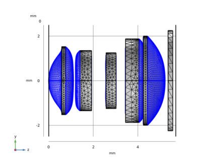
Find the subsection. From the list, choose . The ray tracing algorithm used by the Geometrical Optics interface computes the refracted ray direction based on a discretized geometry via the underlying finite element mesh. A cubic geometry shape order usually introduces less discretization error compared to the default, which uses linear and quadratic polynomials.

Definitions

In the following, create a selection containing the surfaces in 3 of the 4 axially symmetric quadrants of the camera. These will be used during postprocessing.

Box 1

In the toolbar, click

In the window for , locate the section.

From the list, choose .

Locate the section. In the text field, type 0.

In the text field, type 0.

Locate the section. From the list, choose .

Complement 1

In the toolbar, click

In the window for , locate the section.

From the list, choose .

Locate the section. Under , click

In the dialog box, in the list, choose , , , and .

Click .

Materials

Now, define the lens materials. In this tutorial the three lens materials will be assigned a refractive index appropriate for the chosen wavelength. However, the material refractive indices could be defined as a function of wavelength (and temperature) using one of the built-in optical dispersion models.

Material 1 (mat1)

In the window, under right-click and choose .

Select Domains 3 and 4 only.

In the window for , locate the section.

In the table, enter the following settings:


Property	Variable	Value	Unit	Property group
Refractive index, real part	n_iso ; nii = n_iso, nij = 0	nref1	1	Refractive index

Material 2 (mat2)

Right-click and choose .

Select Domains 2, 5, and 6 only.

In the window for , locate the section.

In the table, enter the following settings:


Property	Variable	Value	Unit	Property group
Refractive index, real part	n_iso ; nii = n_iso, nij = 0	nref2	1	Refractive index

Material 3 (mat3)

Right-click and choose .

Select Domain 1 only.

In the window for , locate the section.

In the table, enter the following settings:


Property	Variable	Value	Unit	Property group
Refractive index, real part	n_iso ; nii = n_iso, nij = 0	nref3	1	Refractive index

Geometrical Optics (gop)

In the following sections the physics is defined.

In the window, under click .

In the window for , locate the section.

In the text field, type 0. In this simulation stray light is not being traced, so reflected rays will not be produced at the lens surfaces.

Select the check box. In this simulation, the geometry normals are used to apply the boundary conditions on all refracting surfaces. This is appropriate for the highest accuracy ray traces in single-physics simulations, where the geometry is not deformed.

Locate the section. From the list, choose . It is assumed that the lenses are surrounded by air at room temperature.

Material Discontinuity 1

In the window, under click .

In the window for , locate the section.

From the list, choose .

Ray Properties 1

In the window, click .

In the window for , locate the section.

In the λ0 text field, type lambda.

Obstructions

In the toolbar, click

and choose .

In the window for , type Obstructions in the text field.

Locate the section. From the list, choose .

Image Surface

In the toolbar, click

and choose .

In the window for , type Image Surface in the text field.

Locate the section. From the list, choose .

Release from Grid 1

In the toolbar, click

and choose .

In the window for , locate the section.

From the list, choose .

Specify the qc vector as


0	x
dz*tan(theta1)	y
dz	z

Specify the rc vector as


0	x
0	y
1	z

In the Rc text field, type D_pupil/2.

In the Nc text field, type N_ring.

Locate the section. Specify the L0 vector as


0	x
tan(theta1)	y
1	z

Release from Grid 2

Right-click and choose .

In the window for , locate the section.

Specify the qc vector as


0	x
dz*tan(theta2)	y
dz	z

Locate the section. Specify the L0 vector as


0	x
tan(theta2)	y
1	z

Release from Grid 3

Right-click and choose .

In the window for , locate the section.

Specify the qc vector as


0	x
dz*tan(theta3)	y
dz	z

Locate the section. Specify the L0 vector as


0	x
tan(theta3)	y
1	z

Release from Grid 4

Right-click and choose .

In the window for , locate the section.

Specify the qc vector as


0	x
dz*tan(theta4)	y
dz	z

Locate the section. Specify the L0 vector as


0	x
tan(theta4)	y
1	z

Mesh 1

Next, refine the mesh on the aspheric surfaces.

Free Triangular 1

In the window, under right-click and choose .

In the window for , locate the section.

From the list, choose .

Size 1

Right-click and choose .

In the window for , locate the section.

From the list, choose .

Free Tetrahedral 1

In the window, right-click and choose .

Right-click and choose .

Study 1

Step 1: Ray Tracing

In the window, under click .

In the window for , locate the section.

From the list, choose .

In the text field, type 0 10. The second path length is sufficiently long to ensure that all rays make it to the image surface.

In the toolbar, click

Results

In the following steps the default ray diagram is adjusted to show different aspects of the ray trace. First, define two cut planes which can be used to render the Compact Camera Module cross-section.

Cut Plane 1

In the toolbar, click

In the window for , locate the section.

From the list, choose .

Cut Plane 2

In the toolbar, click

Ray Diagram 1

In the window, under click .

In the window for , type Ray Diagram 1 in the text field.

Ray Trajectories 1

In the window, expand the node.

Color Expression 1

In the window, expand the node, then click .

In the window for , locate the section.

In the text field, type gop.prf. This is the index of each of the release features, starting at 1

Filter 1

In the window, click .

In the window for , locate the section.

From the list, choose .

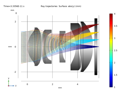
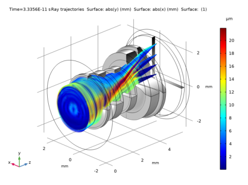
In the text field, type at(0,abs(x))<0.01[mm]. Only the tangential rays will be rendered in this view.

Surface 1

In the window, right-click and choose .

In the window for , locate the section.

From the list, choose .

Locate the section. In the text field, type abs(y).

Locate the section. From the list, choose .

From the list, choose .

Clear the check box.

In the toolbar, click

. Orient the view to match Figure 1 to show only the tangential rays.

Ray Diagram 2

Right-click and choose .

In the window for , type Ray Diagram 2 in the text field.

Locate the section. From the list, choose .

Locate the section. Select the check box.

In the window, expand the node.

Color Expression 1

In the window, expand the node, then click .

In the window for , locate the section.

In the text field, type at('last',gop.rrel). This is the radial coordinate relative to the centroid of each release feature at the image plane.

From the list, choose .

Filter 1

In the window, click .

In the window for , locate the section.

From the list, choose .

Surface 2

In the window, under right-click and choose .

In the window for , locate the section.

From the list, choose .

Locate the section. In the text field, type abs(x).

Surface 3

In the window, right-click and choose .

In the window for , locate the section.

From the list, choose .

Selection 1

Right-click and choose .

In the window for , locate the section.

From the list, choose .

In the toolbar, click

. Orient the view to match Figure 6 to show the all the rays.

Spot Diagram

In the following steps a spot diagram will be created to show the location of the rays in the image plane.

In the toolbar, click

and choose .

In the window for , type Spot Diagram in the text field.

Locate the section. Select the check box.

Spot Diagram 1

In the toolbar, click

and choose .

Color Expression 1

Right-click and choose .

In the window for , locate the section.

In the text field, type at(0,gop.rrel). This is the radial coordinate relative to the centroid at the entrance pupil for each ray release.

In the toolbar, click

Click the

button in the toolbar. Compare the resulting image to Figure 7.

Appendix — Geometry Instructions

From the menu, choose .

New

In the window, click

Model Wizard

In the window, click

Click

Compact Camera Module Geometry Sequence

In the window, under click .

In the window for , type Compact Camera Module Geometry Sequence in the text field.

Locate the section. From the list, choose .

Global Definitions

Parameters 1

In the window, under click .

In the window for , locate the section.

Click

Browse to the model’s Application Libraries folder and double-click the file compact_camera_module_geom_sequence_parameters.txt.

Part Libraries

In the toolbar, click

and choose .

In the window, under click .

In the window, select in the tree.

Click

Compact Camera Module Geometry Sequence

Stop

In the window, under click .

In the window for , type Stop in the text field.

Locate the section. In the table, enter the following settings:


Name	Expression	Value	Description
d0	d0_S	5 mm	Diameter, outer
d1	d1_S	2.505 mm	Diameter, inner
nix	nix	0	Local optical axis, x-component
niy	niy	0	Local optical axis, y-component
niz	niz	1	Local optical axis, z-component

Click to expand the section. In the table, select the check box for .

Click to select row number 1 in the table.

Click .

In the dialog box, type Aspheric Surfaces in the text field.

Click . This selection will be used to to refine the mesh on the aspheric surfaces.

In the window for , locate the section.

Click .

In the dialog box, type Obstructions in the text field.

Click .

Part Libraries

In the toolbar, click

and choose .

In the window, click .

In the window, select in the tree.

Click

In the dialog box, select in the list.

Click .

Compact Camera Module Geometry Sequence

Lens 1

In the window, under click .

In the window for , type Lens 1 in the text field.

Locate the section. Click

Browse to the model’s Application Libraries folder and double-click the file compact_camera_module_geom_sequence_lens1.txt. These files are simplify the mapping between the lens prescription and the input parameters for this part. Similar files will be used for each of the four remaining lenses.

Locate the section. In the table, enter the following settings:


Name	Keep	Physics	Contribute to
Exterior	√	√	None
Surface 1		√	Aspheric Surfaces
Surface 2		√	Aspheric Surfaces
Edges		√	Obstructions

Lens 2

In the toolbar, click

and choose .

In the window for , type Lens 2 in the text field.

Locate the section. Click

Browse to the model’s Application Libraries folder and double-click the file compact_camera_module_geom_sequence_lens2.txt.

Locate the section. Find the subsection. From the list, choose .

From the list, choose .

Find the subsection. In the text field, type T_1.

Locate the section. In the table, enter the following settings:


Name	Keep	Physics	Contribute to
Exterior	√	√	None
Surface 1		√	Aspheric Surfaces
Surface 2		√	Aspheric Surfaces
Edges		√	Obstructions

Lens 3

In the toolbar, click

and choose .

In the window for , type Lens 3 in the text field.

Locate the section. Click

Browse to the model’s Application Libraries folder and double-click the file compact_camera_module_geom_sequence_lens3.txt.

Locate the section. Find the subsection. From the list, choose .

From the list, choose .

Find the subsection. In the text field, type T_2.

Locate the section. In the table, enter the following settings:


Name	Keep	Physics	Contribute to
Exterior	√	√	None
Surface 1		√	Aspheric Surfaces
Surface 2		√	Aspheric Surfaces
Edges		√	Obstructions

Lens 4

In the toolbar, click

and choose .

In the window for , type Lens 4 in the text field.

Locate the section. Click

Browse to the model’s Application Libraries folder and double-click the file compact_camera_module_geom_sequence_lens4.txt.

Locate the section. Find the subsection. From the list, choose .

From the list, choose .

Find the subsection. In the text field, type T_3.

Locate the section. In the table, enter the following settings:


Name	Keep	Physics	Contribute to
Exterior	√	√	None
Surface 1		√	Aspheric Surfaces
Surface 2		√	Aspheric Surfaces
Edges		√	Obstructions

Lens 5

In the toolbar, click

and choose .

In the window for , type Lens 5 in the text field.

Locate the section. Click

Browse to the model’s Application Libraries folder and double-click the file compact_camera_module_geom_sequence_lens5.txt.

Locate the section. Find the subsection. From the list, choose .

From the list, choose .

Find the subsection. In the text field, type T_4.

Locate the section. In the table, enter the following settings:


Name	Keep	Physics	Contribute to
Exterior	√	√	None
Surface 1		√	Aspheric Surfaces
Surface 2		√	Aspheric Surfaces
Edges		√	Obstructions

Part Libraries

In the toolbar, click

and choose .

In the window, click .

In the window, select in the tree.

Click

In the dialog box, select in the list.

Click .

Compact Camera Module Geometry Sequence

IR Filter

In the window, under click .

In the window for , type IR Filter in the text field.

Locate the section. In the table, enter the following settings:


Name	Expression	Value	Description
R1	0	0 m	Radius of curvature, surface 1 (+convex/-concave)
R2	0	0 m	Radius of curvature, surface 2 (-convex/+concave)
Tc	Tc_F	0.21 mm	Center thickness
d0	d0_F	4.5 mm	Lens full diameter
d1	0	0 m	Diameter, surface 1
d2	0	0 m	Diameter, surface 2
d1_clear	0	0 m	Clear aperture diameter, surface 1
d2_clear	0	0 m	Clear aperture diameter, surface 2

Locate the section. Find the subsection. From the list, choose .

From the list, choose .

Find the subsection. In the text field, type T_5.

Locate the section. In the table, enter the following settings:


Name	Keep	Physics	Contribute to
Exterior	√	√	None
Edges		√	Obstructions

Image Plane

In the toolbar, click

and choose .

In the window for , type Image Plane in the text field.

Locate the section. In the table, enter the following settings:


Name	Expression	Value	Description
d0	d0_I	5 mm	Diameter, outer
d1	0	0 m	Diameter, inner

Locate the section. Find the subsection. From the list, choose .

From the list, choose .

Find the subsection. In the text field, type T_6.

Locate the section. In the table, select the check box for .

In the toolbar, click

Click the

button in the toolbar. Orient the view to place the optical axis (z-axis) horizontal and the y-axis vertical. Compare the resulting geometry to Figure 2.

This level of mesh refinement is only needed for certain surface types. The default physics-controlled mesh is often suitable for single physics ray tracing studies when using the high-accuracy surfaces used in the spherical and conic lens and mirror parts from the Ray Optics Module Part Libraries.