Waveguide Iris Bandpass Filter

A conductive diaphragm, an iris, placed transverse to a waveguide aperture causes a discontinuity and generates shunt reactance. Bandpass frequency response can be achieved from cascaded cavity resonators combined with such reactive elements, which can be created by inserting a series of iris elements inside the waveguide. This example consists of a WR-90 X-band waveguide and symmetrical inductive diaphragms (irises). The calculated S-parameters show good bandpass response and out-of-band rejection.

Figure 1: Symmetrical irises inside the waveguide generate shunt inductance. The top surface is removed to show the inside.

Model Definition

This example uses a WR-90 waveguide for X-band applications. The waveguide and iris parts are modeled as perfect electric conductors (PECs) and the inside of the waveguide is filled with air. On each end of the waveguide, a port boundary condition is applied with the predefined rectangular TE10 mode. Only one port is excited to observe the S-parameters of the example. The upper cut-off frequency can be approximately estimated using the resonant frequency of the biggest cavity located in the middle of the filter via

where a and b are the dimensions of the waveguide’s aperture and d is the length of the cavity. For this example, the values a = 2.286 cm, b = 1.016 cm, and d = 1.73 cm give a resonant frequency at the dominant mode, TE101, of 10.87 GHz. Because the cavities are not completely closed but formed with the open irises, this estimation gives only an approximated value.

Results and Discussion

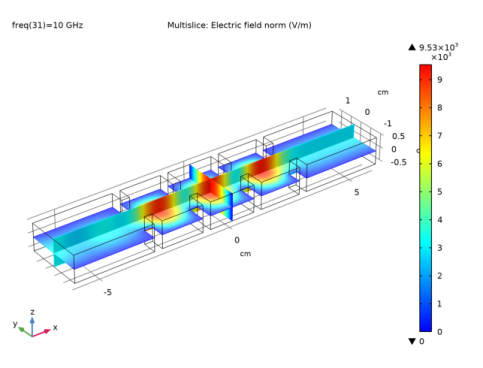
The default plot shows the norm of the electric fields in the waveguide; see Figure 2. At 10 GHz, the shape of the field distribution in each section of cavities looks like that of the dominant mode of a cavity.

Figure 2: The E-field norm plot at the passband frequency shows the dominant mode resonance in each cavity formed by the irises.

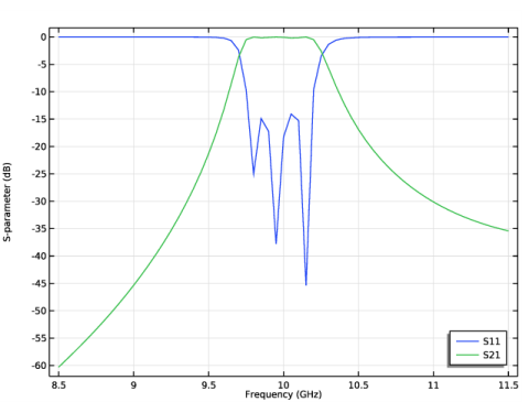
Figure 3 shows the calculated S-parameters. The passband is around 10 GHz and good out-of-band rejection frequency response is observed.

Figure 3: The calculated S-parameters show good matching characteristics as well as out-of-band rejection.

In Figure 4, the calculated S-parameters from the Frequency Domain, Modal method are plotted together with those of the discrete frequency sweep. While the frequency resolution of the Frequency Domain, Modal is five times finer than that of the discrete frequency sweep, the simulation time is four times faster to analyze the same filter.

Figure 4: The calculated S-parameters from the Frequency Domain, Modal method are plotted with those of the discrete frequency sweep (dashed lines with circle makers).

References

1. D.M. Pozar, Microwave Engineering, John Wiley & Sons, 1998.

2. R.E. Collin, Foundation of Microwave Engineering, McGraw-Hill, 1992.

RF_Module/Filters/waveguide_iris_filter

Modeling Instructions

From the menu, choose .

New

In the window, click

Model Wizard

In the window, click

In the tree, select .

Click .

Click

In the tree, select .

Click

Study 1

Step 1: Frequency Domain

In the window, under click .

In the window for , locate the section.

Click

In the dialog box, type 8.5[GHz] in the text field.

In the text field, type 0.05[GHz].

In the text field, type 11.5[GHz].

Click .

Global Definitions

Parameters 1

In the window, under click .

In the window for , locate the section.

Click

Browse to the model’s Application Libraries folder and double-click the file waveguide_iris_filter_parameters.txt.

Geometry 1

In the window, under click .

In the window for , locate the section.

From the list, choose .

Create a block for the WR-90 waveguide.

WR-90

In the toolbar, click

In the window for , type WR-90 in the text field.

Locate the section. In the text field, type 12.

In the text field, type w_wg.

In the text field, type h_wg.

Locate the section. From the list, choose .

Click

Choose wireframe rendering to get a view inside the waveguide when adding the irises.

Click the

button in the toolbar.

Next, add a block for generating the inner irises, which form the center cavity.

Iris1

In the toolbar, click

In the window for , type Iris1 in the text field.

Locate the section. In the text field, type d_iris.

In the text field, type l_iris1.

In the text field, type h_wg.

Locate the section. From the list, choose .

In the text field, type spacing/2.

In the text field, type (w_wg-l_iris1)/2.

Add another block for generating the outer irises, which enclose the first and last cavities.

Iris2

In the toolbar, click

In the window for , type Iris2 in the text field.

Locate the section. In the text field, type d_iris.

In the text field, type l_iris2.

In the text field, type h_wg.

Locate the section. From the list, choose .

In the text field, type spacing*1.42.

In the text field, type (w_wg-l_iris2)/2.

Click

Create symmetrical inductive diaphragms by mirroring the iris blocks a couple of times.

Mirror 1 (mir1)

In the toolbar, click

and choose .

Select the objects and only.

In the window for , locate the section.

Select the check box.

Locate the section. In the text field, type 1.

In the text field, type 0.

Mirror 2 (mir2)

In the toolbar, click

and choose .

Select the objects , , , and only.

In the window for , locate the section.

Select the check box.

Locate the section. In the text field, type 1.

In the text field, type 0.

Difference 1 (dif1)

In the toolbar, click

and choose .

Select the object only.

In the window for , locate the section.

Find the subsection. Select the

toggle button.

Select the objects , , , , , , , and only.

Click

Electromagnetic Waves, Frequency Domain (emw)

Now, set up the physics. The default boundary condition, Perfect Electric Conductor, applies to all exterior boundaries.

Port 1

In the window, under right-click and choose .

Select Boundary 1 only.

The excitation port

In the window for , locate the section.

From the list, choose .

For the first port, wave excitation is by default.

Port 2

In the toolbar, click

and choose .

Select Boundary 38 only.

The observation port

In the window for , locate the section.

From the list, choose .

Materials

Assign material properties on the model. Use air for all domains.

Add Material

In the toolbar, click

to open the window.

Go to the window.

In the tree, select .

Click in the window toolbar.

In the toolbar, click

to close the window.

Mesh 1

In the window, under right-click and choose .

Study 1

In the toolbar, click

Results

Electric Field (emw)

The default plot shows the distribution of the norm of the electric field. Choose the center frequency of the passband.

In the window for , locate the section.

From the list, choose .

In the toolbar, click

The resonant E-field should be observed in the cavities. Compare with Figure 2.

S-parameter (emw)

In the window, click .

In the window for , locate the section.

From the list, choose .

In the toolbar, click

The resulting plot shows the S-parameters of the filter. Compare the plot with Figure 3.

Smith Plot (emw)

Analyze the same model with a Frequency Domain Modal method. When a device presents resonances, the method combined with an analysis provides a faster solution time.

Add Study

In the toolbar, click

to open the window.

Go to the window.

Find the subsection. In the tree, select .

Click in the window toolbar.

In the toolbar, click

to close the window.

Study 2

Step 1: Eigenfrequency

In the window for , locate the section.

In the text field, type 9.5[GHz].

Step 2: Frequency Domain, Modal

In the window, click .

In the window for , locate the section.

In the text field, type range(8.5[GHz],0.01[GHz],11.5[GHz]).

With a very fine frequency step simulation, the solutions contain a lot of data. As a result, the model file size will increase tremendously when it is saved. By selecting the Store fields in output check box in the Values of Dependent Variables section of the Frequency Domain study step settings, it is possible to define for what part of the model the computed solution should be saved. When only S-parameters are of interest, it is not necessary to store all of the field solutions. Instead, only store the field on the selections for the port boundaries, as those will be used for the S-parameter calculations.

Electromagnetic Waves, Frequency Domain (emw)

Port 1

In the window, under click .

In the window for , locate the section.

Click

In the dialog box, type Port 1 in the text field.

Click .

Port 2

In the window, click .

In the window for , locate the section.

Click

In the dialog box, type Port 2 in the text field.

Click .

Study 2

Step 2: Frequency Domain, Modal

In the window, under click .

In the window for , click to expand the section.

Find the subsection. From the list, choose .

Under , click

In the dialog box, in the list, choose and .

Click .

It is necessary to include the port boundaries to calculate S-parameters. By choosing only the port boundaries for settings, it is possible to reduce the size of a model file a lot.

In the toolbar, click

Results

Multislice

In the window, expand the node, then click .

In the window for , locate the section.

Find the subsection. From the list, choose .

In the text field, type -6 6.

Find the subsection. In the text field, type 0.

In the toolbar, click

Since 11.5 GHz is not within the passband, the input power at the excitation port is not delivered to the observation port.

Electric Field (emw) 1

In the window, click .

In the window for , locate the section.

From the list, choose .

In the toolbar, click

When the frequency of the plot is within the passband, the input power at the excitation port is delivered to the observation port.

Next, plot the calculated S-parameters from the Frequency Domain Modal method together with those of the discrete frequency sweep.

S-parameter (emw) 1

In the window, click .

In the window for , locate the section.

From the list, choose .

Global 1

In the window, expand the node, then click .

In the window for , locate the section.

In the table, enter the following settings:


Expression	Unit	Description
emw.S11dB	1	S11 Frequency Domain Modal
emw.S21dB	1	S21 Frequency Domain Modal

Global 2

In the window, right-click and choose .

In the window for , locate the section.

From the list, choose .

Click in the upper-right corner of the section. From the menu, choose .

Locate the section. In the table, enter the following settings:


Expression	Unit	Description
emw.S11dB	1	S11 Regular Sweep
emw.S21dB	1	S21 Regular Sweep

Click to expand the section. Find the subsection. From the list, choose .

Find the subsection. From the list, choose .

From the list, choose .

In the toolbar, click

S-parameter (emw) 1

In the window, click .

In the window for , click to expand the section.

From the list, choose .

In the text area, type S-parameter Comparison between Frequency Domain Modal and Regular Discrete Sweep.

Compare the plot with Figure 4.

Smith Plot (emw) 1

Analyze the same model with a finer frequency resolution using based on asymptotic waveform evaluation (AWE). When a device presents a slowly varying frequency response, the AWE provides a faster solution time when running the simulation on many frequency points. The following example with the AWE can be computed five times faster than regular Frequency Domain sweeps with a same finer frequency resolution.

Add Study

In the toolbar, click