Fast Modeling of a Transmission Line Low-Pass Filter

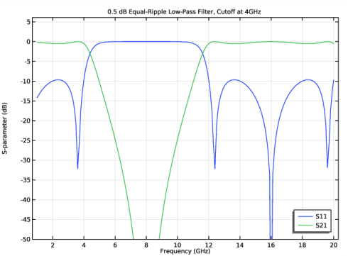
One way to design a filter is to utilize the element values of well-known filter prototypes such as maximally flat or equal-ripple low-pass filters. It is easier to fabricate a distributed element filter on a microwave substrate than a lumped element filter since it is cumbersome to find off-the-shelf capacitors and inductors exactly matched to the frequency-scaled element values of the filter prototype. This example demonstrates the design process of a distributed element filter using Richard’s transformation, Kuroda’s identity, and the Transmission Line physics interface. This approach is very fast compared to solving Maxwell’s equations in 3D. The model simulates a three-element 0.5 dB equal-ripple low-pass filter that has a cutoff frequency at 4 GHz. The resulting S-parameter plot shows a low-pass frequency response that is also periodically observed at higher frequency range.

Figure 1: Microstrip low-pass filter circuit. The impedance for each unit length (0.125 wavelengths) stub is calculated from the element values of a three element 0.5 dB equal-ripple low-pass filter.

Model Definition

The modeling process of a low-pass filter can be summarized as

•

Define a filter type such as maximally flat or equal-ripple.

•

Identify element values for the filter prototype.

•

Convert the inductors and capacitors in the lumped element filter to series and shunt stubs by using Richard’s transformation.

•

Apply Kuroda’s identity to convert short-circuited series stubs to open-circuited shunt stubs.

•

Scale the impedance of stubs by the reference characteristic impedance (50 Ω) and set the length of stubs to 0.125 wavelengths defined by the cutoff frequency.

Ref. 1 provides the element values for a 0.5 dB equal-ripple low-pass filter. The element values for a three element prototype are also shown in Table 1.

Table 1: 0.5 decibel Equal-Ripple low-pass filter element values, N = 3.
g1	g2	g3	g4
1.5963	1.0967	1.5963	1

These values are unscaled inductance and capacitance in a lumped element circuit that need to be converted to distributed elements. Richard’s transformation converts an inductor to a short-circuited stub and a capacitor to an open-circuited stub, respectively. The model is based on a three element prototype beginning with a series inductor. Two series inductors are transformed to series stubs and one shunt capacitor is transformed to a shunt stub. The normalized impedance of the open-circuited stub is the same as the lumped element value of the inductor (Equation 1) and that for the short-circuited stub is the inverse of the lumped element value of the capacitor (Equation 2).

(1)

(2)

The short-circuited series stub is not easily realizable as a microstrip circuit so it has to be transformed again using Kuroda’s identity that will convert a short-circuited series to an open-circuited shunt stub. A unit length (0.125 wavelengths) transmission line element must be added at each end of the input and output of the filter before applying Kuroda’s identity. During this transformation, the impedance of the stub and an additional unit length microstrip line element is scaled by n2 (Equation 3).

(3)

(4)

(5)

The location of the converted open-circuited stub and the added unit length microstrip line element is swapped to complete the filter geometry. Finally, the impedance is scaled by the reference characteristic impedance, 50 Ω.

Figure 2: The three element filter design using lumped element prototype element values.

The filter geometry is built with six lines (Bézier polygons) on a two-dimensional space. The properties of each line representing a microstrip line with a different characteristic impedance are configured by Transmission Line Equation features.

The transmission line parameters for a 50 Ω microstrip line built on a 20 mil lossless substrate with permittivity εr = 3.38 and 1 oz copper can be calculated accurately from Ref. 2.

Table 2: Calculated transmission line parameters of a 50 Ω microstrip line.
R	L	G	C
12.41 Ω/m	272.9 nH/m	0 S/m	107.1 pF/m

The contribution of the distributed resistance on the insertion loss with the given substrate properties is less than 0.05 dB. To make the modeling steps simpler in this example, the approximated parameter values in Table 3 are used for a 50 Ω microstrip line.

Table 3: simplified transmission line parameters of a 50 Ω microstrip line.
R	L	G	C
0 Ω/m	250 nH/m	0 S/m	100 pF/m

Other transmission line parameters with different characteristic impedance values are adjusted using the normalized impedance. The distributed inductance is proportionally scaled and the distributed capacitance is inversely scaled by the normalized impedance of the microstrip line.

Results and Discussion

The S-parameters, S11 and S21, of the low-pass filter are plotted in Figure 3. The cutoff is shown at the intended frequency of 4 GHz. The ripple of S21 is 0.5 dB.