PDF

RF Coil
Introduction
RF coils are important in numerous applications, ranging from wireless technology to MRI scanning equipment. This introductory tutorial model demonstrates how to find the fundamental resonance frequency of a coil, and perform a frequency sweep to extract its Q-factor.
Model Definition
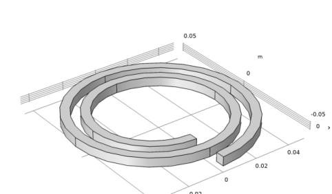
The considered coil consists of two turns, as shown in Figure 1. In the first version of the example, this geometry is used in finding the fundamental resonance. The coil is considered to be a perfect electric conductor, which means you need to solve the eigenfrequency equation for the electromagnetic waves only in its surrounding air. The air domain is a sphere sufficiently large that its exterior boundary conditions do not considerably affect the solution.
Figure 1: Geometry used for the eigenfrequency analysis.
In the second version of the example, a time-harmonic driving port voltage is assigned between the two ends of the coil. This is accomplished by connecting them through a lumped port (see Lumped Ports with Voltage Input in the RF Module User’s Guide). The port is assigned a 50 Ω external cable impedance and a 1 V driving voltage. The model is run through a range of frequencies surrounding the resonance.
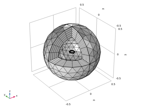
In order to let the generated waves leave the model domain with a minimum of artificial reflections, the driven version of the example has a PML outside the air sphere. Figure 2 shows the meshed geometry.
The driven model considers the coil as made of copper. It accounts for the conductive surface losses with the help of an Impedance Boundary Condition (see the RF Module User’s Guide).
Figure 2: The mesh used in the driven version of the example. A slice is cut out and the air domain made invisible in order to show the coil.
Results and Discussion
The eigenfrequency version of the example finds the lowest eigenfrequency at 180 MHz. In order to verify that the air sphere is sufficiently large, this result is confirmed with the artificial exterior boundaries set first to perfect electric conductors, then to perfect magnetic conductors. Figure 3 shows the distribution of the electric and magnetic fields at this resonance.
Figure 3: Electric field (slice) and magnetic flux density (arrows) at the fundamental resonance.
The lumped port condition in the driven problem automatically provides the impedance of the example. This is the input impedance to the cable; as such it is independent of the 50 Ω cable impedance. Plotting the impedance versus the frequency lets you evaluate the Q-factor of the device:
,
where f0 is the peak frequency and Δf the full width at half maximum, as seen in Figure 4.
 
Figure 4: Input impedance versus frequency. The Q-value evaluates to approximately 400.
Application Library path: RF_Module/Passive_Devices/rf_coil
Modeling Instructions
From the File menu, choose New.
New
In the New window, click  Model Wizard.
Model Wizard
1
In the Model Wizard window, click  3D.
2
In the Select Physics tree, select Radio Frequency>Electromagnetic Waves, Frequency Domain (emw).
3
Click Add.
4
Click  Study.
Begin with the Eigenfrequency study. You add another Frequency Domain study later.
5
In the Select Study tree, select General Studies>Eigenfrequency.
6
Geometry 1
Import 1 (imp1)
1
In the Home toolbar, click  Import.
2
In the Settings window for Import, locate the Import section.
3
Click Browse.
4
5
Click Import.
Create an air sphere surrounding the coil.
Sphere 1 (sph1)
1
In the Geometry toolbar, click  Sphere.
2
In the Settings window for Sphere, locate the Size section.
3
In the Radius text field, type 0.25.
4
Click  Build All Objects.
5
Click the  Zoom Extents button in the Graphics toolbar.
6
Click the  Transparency button in the Graphics toolbar.
Add Material
1
In the Home toolbar, click  Add Material to open the Add Material window.
2
Go to the Add Material window.
3
4
Click Add to Component in the window toolbar.
5
In the Home toolbar, click  Add Material to close the Add Material window.
Materials
Air (mat1)
The first material that you choose, in this case air, by default applies to all domains. This is fine, as you are anyway going to exclude the interior of the coil from the model in the next step.
Electromagnetic Waves, Frequency Domain (emw)
1
In the Model Builder window, under Component 1 (comp1) click Electromagnetic Waves, Frequency Domain (emw).
2
With the coil domain removed from the model, the coil surface will by default get the Perfect Electric Conductor boundary condition. This will also apply to the exterior boundaries of the air domain.
Given that the air domain is sufficiently large, the condition on its exterior boundaries should have a limited effect on the result. To verify that this is the case, you will solve this model once with the default Perfect Electric Conductor condition and once with the Perfect Magnetic Conductor condition. The difference between the resulting eigenfrequencies will give you an idea of the accuracy of the results, and the mean of the two solutions should be a good estimate of the actual value.
Mesh 1
Free Tetrahedral 1
In the Mesh toolbar, click  Free Tetrahedral.
Size 1
1
Right-click Free Tetrahedral 1 and choose Size.
2
In the Settings window for Size, locate the Geometric Entity Selection section.
3
From the Geometric entity level list, choose Domain.
4
5
Locate the Element Size section. From the Predefined list, choose Fine.
6
Click the Custom button.
7
Locate the Element Size Parameters section. Select the Maximum element size check box.
8
The 5 mm maximum element size in the coil domain helps you get a relatively uniform mesh in the vicinity of the coil.
9
Click  Build All.
Study 1
Step 1: Eigenfrequency
By default, the eigenfrequency solver will return six eigenfrequencies. However, by requesting only one eigenfrequency, the solver will only return the true physical solution around 180 MHz and not the lower frequency spurious solutions.
1
In the Model Builder window, under Study 1 click Step 1: Eigenfrequency.
2
In the Settings window for Eigenfrequency, locate the Study Settings section.
3
In the Search for eigenfrequencies around text field, type 180[MHz].
4
Select the Desired number of eigenfrequencies check box.
5
6
In the Home toolbar, click  Compute.
Results
Electric Field (emw)
The Eigenfrequency list should contain a solution of the order of 180 MHz. If the eigenfrequency in the list is something else, the solver has probably returned a spurious solution. If you suspect that the solver has returned a spurious solution, it helps to plot the fields and verify that the solution contains only noise. In that case, redo the calculation with more eigenfrequencies and select the eigenfrequency around 180 MHz. For now, display a slice plot of the electric field distribution for the eigenfrequency around 180 MHz.
Replace the Multislice plot with a single slice.
Multislice
1
In the Model Builder window, expand the Electric Field (emw) node.
2
Right-click Multislice and choose Delete.
Slice 1
1
In the Model Builder window, right-click Electric Field (emw) and choose Slice.
2
In the Settings window for Slice, locate the Plane Data section.
3
From the Plane list, choose XY-planes.
4
In the Planes text field, type 1.
5
In the Electric Field (emw) toolbar, click  Plot.
6
Click the  Transparency button in the Graphics toolbar.
7
Click the  Zoom In button in the Graphics toolbar.
8
Click the  Zoom In button in the Graphics toolbar.
It is clear that the electric field is much greater between the turns of the coil than anywhere else. You can get a better view of the distribution within the coil by adjusting the range a little. Add an arrow plot of the magnetic flux density to reproduce Figure 3.
9
Click to expand the Range section. Select the Manual color range check box.
10
In the Minimum text field, type 500.
11
In the Maximum text field, type 2000.
12
In the Electric Field (emw) toolbar, click  Plot.
Arrow Volume 1
1
Right-click Electric Field (emw) and choose Arrow Volume.
2
In the Settings window for Arrow Volume, click Replace Expression in the upper-right corner of the Expression section. From the menu, choose Component 1 (comp1)>Electromagnetic Waves, Frequency Domain>Magnetic>emw.Bx,...,emw.Bz - Magnetic flux density.
The selection you just made would give you an arrow plot of the real part of the magnetic flux density. Because the magnetic fields are 90 degrees out of phase with the electric potential applied by the port, that evaluates to zero. Adjust the expressions manually to look at the imaginary part instead.
3
Locate the Expression section. In the X component text field, type imag(emw.Bx).
4
In the Y component text field, type imag(emw.By).
5
In the Z component text field, type imag(emw.Bz).
6
Locate the Arrow Positioning section. Find the X grid points subsection. In the Points text field, type 45.
7
Find the Y grid points subsection. In the Points text field, type 45.
8
Find the Z grid points subsection. In the Points text field, type 10.
9
Locate the Coloring and Style section. From the Color list, choose White.
10
In the Electric Field (emw) toolbar, click  Plot.
These are all the exterior boundaries of the air domain.
Electromagnetic Waves, Frequency Domain (emw)
Perfect Magnetic Conductor 1
1
In the Physics toolbar, click  Boundaries and choose Perfect Magnetic Conductor.
2
Click the  Zoom Extents button in the Graphics toolbar.
3
Study 1
In the Home toolbar, click  Compute.
Results
Electric Field (emw)
1
In the Electric Field (emw) toolbar, click  Plot.
The fundamental eigenfrequency is now slightly lower than before. The difference is so small that the numerical error due to the finite mesh is likely greater than the systematic error due to the outer boundary condition.
In the driven problem, not only the resonance frequency but also the radiation losses are important. These are better captured if the size of the geometry is of the same order of magnitude as the wavelength. Because the driven analysis uses a highly memory-efficient iterative solver, you can afford to increase the size of the sphere a little.
Geometry 1
Sphere 1 (sph1)
1
In the Model Builder window, under Component 1 (comp1)>Geometry 1 click Sphere 1 (sph1).
2
In the Settings window for Sphere, locate the Size section.
3
In the Radius text field, type 0.5.
First, add a PML layer to the sphere.
4
Click to expand the Layers section. In the table, enter the following settings:
5
Click the  Wireframe Rendering button in the Graphics toolbar.
Next, create a work plane to draw and embed rectangles for your excitation port.
Work Plane 1 (wp1)
1
In the Geometry toolbar, click  Work Plane.
2
In the Settings window for Work Plane, locate the Plane Definition section.
3
From the Plane list, choose yz-plane.
4
Click  Show Work Plane.
Work Plane 1 (wp1)>Plane Geometry
1
Click the  Zoom Extents button in the Graphics toolbar.
2
Click the  Zoom In button in the Graphics toolbar.
Work Plane 1 (wp1)>Rectangle 1 (r1)
1
In the Work Plane toolbar, click  Rectangle.
2
In the Settings window for Rectangle, locate the Size and Shape section.
3
In the Width text field, type 5e-3.
4
In the Height text field, type 15e-3.
5
Locate the Position section. In the xw text field, type -0.05.
6
In the yw text field, type -0.0175.
Work Plane 1 (wp1)>Rectangle 2 (r2)
1
In the Work Plane toolbar, click  Rectangle.
2
In the Settings window for Rectangle, locate the Size and Shape section.
3
In the Width text field, type 5e-3.
4
In the Height text field, type 15e-3.
5
Locate the Position section. In the xw text field, type -0.03.
6
In the yw text field, type -0.0175.
Work Plane 1 (wp1)>Rectangle 3 (r3)
1
In the Work Plane toolbar, click  Rectangle.
2
In the Settings window for Rectangle, locate the Size and Shape section.
3
In the Width text field, type 15e-3.
4
In the Height text field, type 5e-3.
5
Locate the Position section. In the xw text field, type -0.045.
6
In the yw text field, type -0.0175.
7
In the Work Plane toolbar, click  Build All.
Form Union (fin)
In the Home toolbar, click  Build All.
Definitions
The driven version of the model will use an impedance boundary condition to take into account the conduction losses in the coil. Define a selection to facilitate this process.
Coil Surface
1
In the Definitions toolbar, click  Explicit.
2
In the Settings window for Explicit, type Coil Surface in the Label text field.
3
Domain 6 is the coil.
4
Locate the Output Entities section. From the Output entities list, choose Adjacent boundaries.
Add Material
1
In the Home toolbar, click  Add Material to open the Add Material window.
2
Go to the Add Material window.
3
In the tree, select Built-in>Copper.
4
Click Add to Component in the window toolbar.
5
In the Home toolbar, click  Add Material to close the Add Material window.
Materials
Copper (mat2)
1
In the Settings window for Material, locate the Geometric Entity Selection section.
2
From the Geometric entity level list, choose Boundary.
3
From the Selection list, choose Coil Surface.
Electromagnetic Waves, Frequency Domain (emw)
Impedance Boundary Condition 1
1
In the Physics toolbar, click  Boundaries and choose Impedance Boundary Condition.
2
In the Settings window for Impedance Boundary Condition, locate the Boundary Selection section.
3
From the Selection list, choose Coil Surface.
4
In the Model Builder window, click Electromagnetic Waves, Frequency Domain (emw).
5
In the Settings window for Electromagnetic Waves, Frequency Domain, locate the Domain Selection section.
6
From the Selection list, choose All domains.
7
While the Perfect Electric Conductor condition is the default on exterior boundaries, you need to apply it manually should you need it on interior ones.
Perfect Electric Conductor 2
1
In the Physics toolbar, click  Boundaries and choose Perfect Electric Conductor.
2
Boundaries 30 and 37 are those connecting the port with the coil.
Lumped Port 1
1
In the Physics toolbar, click  Boundaries and choose Lumped Port.
2
Boundary 33 connects the two perfect electric conductors you just defined.
For the first port, wave excitation is on by default.
3
In the Settings window for Lumped Port, locate the Boundary Selection section.
4
Click  Create Selection.
Create a set of selections for use in the study settings.
5
In the Create Selection dialog box, type Lumped port 1 in the Selection name text field.
6
Definitions
Perfectly Matched Layer 1 (pml1)
1
In the Definitions toolbar, click  Perfectly Matched Layer.
2
3
In the Settings window for Perfectly Matched Layer, locate the Geometry section.
4
From the Type list, choose Spherical.
Mesh 1
When setting up the mesh for the driven problem, make sure to get a fine mesh on the port boundary. The PML performs at its best when it is meshed with a swept mesh.
Size
1
In the Model Builder window, under Component 1 (comp1)>Mesh 1 click Size.
2
In the Settings window for Size, locate the Element Size section.
3
Click the Custom button.
4
Locate the Element Size Parameters section. In the Minimum element size text field, type 0.003.
Free Tetrahedral 1
1
In the Model Builder window, click Free Tetrahedral 1.
2
In the Settings window for Free Tetrahedral, locate the Domain Selection section.
3
From the Geometric entity level list, choose Domain.
4
Domain 5 is the coil and Domain 6 the surrounding air domain.
Size 1
1
In the Model Builder window, click Size 1.
2
Size 2
1
In the Model Builder window, right-click Free Tetrahedral 1 and choose Size.
2
In the Settings window for Size, locate the Geometric Entity Selection section.
3
From the Geometric entity level list, choose Boundary.
4
Boundary 33 is the port boundary.
5
Locate the Element Size section. From the Predefined list, choose Finer.
6
Click the Custom button.
7
Locate the Element Size Parameters section. Select the Maximum element size check box.
8
Swept 1
In the Mesh toolbar, click  Swept.
Distribution 1
1
Right-click Swept 1 and choose Distribution.
The default 5 elements is a sufficient number to have across the PML.
2
Right-click Distribution 1 and choose Build All.
Definitions
Hide for Physics 1
1
In the Model Builder window, right-click View 1 and choose Hide for Physics.
2
Domain 2 is the PML domain straight in front of you if you are in the default coordinate system view, but any one of the outer domains will do.
Hide for Physics 2
1
Right-click View 1 and choose Hide for Physics.
2
In the Settings window for Hide for Physics, locate the Geometric Entity Selection section.
3
From the Geometric entity level list, choose Boundary.
4
Mesh 1
Compare the meshed structure with the above figure.
5
Click the  Reset Hiding button in the Graphics toolbar.
Add Study
1
In the Home toolbar, click  Add Study to open the Add Study window.
2
Go to the Add Study window.
3
Find the Studies subsection. In the Select Study tree, select Preset Studies for Selected Physics Interfaces>Adaptive Frequency Sweep.
4
Click Add Study in the window toolbar.
5
In the Home toolbar, click  Add Study to close the Add Study window.
Study 2
Step 1: Adaptive Frequency Sweep
1
In the Settings window for Adaptive Frequency Sweep, locate the Study Settings section.
2
In the Frequencies text field, type range(173[MHz],0.01[MHz],175.2[MHz]).
This gives you a range of frequencies starting at 173 MHz and ending at 175.2 MHz, with a solution at every 0.01 MHz.
3
From the AWE expression type list, choose User controlled.
4
A slowly varying scalar value curve works well for AWE expressions. Use abs(comp1.emw.Zport_1) for this coil model.
Because such a fine frequency step generates a memory-intensive solution, the model file size will increase tremendously when it is saved. When only the frequency response of port related variables are of interest, it is not necessary to store all of the field solutions. By selecting the Store fields in output check box in the Values of Dependent Variables section, we can control the part of the model on which the computed solution is saved. We only add the selection containing these boundaries where the port variables are calculated. The lumped port size is typically very small compared to the entire modeling domain, and the saved file size with the fine frequency step is more or less that of the regular discrete frequency sweep model when only the solutions on the port boundaries are stored.
5
Locate the Values of Dependent Variables section. Find the Store fields in output subsection. From the Settings list, choose For selections.
6
Under Selections, click  Add.
7
In the Add dialog box, select Lumped port 1 in the Selections list.
8
9
In the Home toolbar, click  Compute.
Results
Electric Field (emw) 1
Since the results are stored only on the lumped port boundaries, this default E-field norm plot does not provide useful information.
1
Right-click Results>Electric Field (emw) 1 and choose Delete.
Set up a 1D plot group to plot the port impedance versus the frequency.
1D Plot Group 5
1
In the Home toolbar, click  Add Plot Group and choose 1D Plot Group.
2
In the Settings window for 1D Plot Group, locate the Data section.
3
From the Dataset list, choose Study 2/Solution 2 (sol2).
4
Click to expand the Title section. From the Title type list, choose Manual.
5
In the Title text area, type Lumped Port Impedance ([Omega]).
6
Locate the Legend section. Clear the Show legends check box.
Global 1
1
Right-click 1D Plot Group 5 and choose Global.
2
In the Settings window for Global, locate the y-Axis Data section.
3
4
Locate the x-Axis Data section. From the Parameter list, choose Expression.
5
In the Expression text field, type freq.
6
From the Unit list, choose MHz.
7
In the 1D Plot Group 5 toolbar, click  Plot.
The impedance peak indicates that the driven problem has its resonance shifted slightly down, to approximately 174 MHz. Compare the reproduced plot with that in Figure 4, from which you can evaluate the Q-factor.