PDF

Rat-Race Coupler
Introduction
A 180° Ring Hybrid (Rat-Race Coupler) is a four-port network with 180° phase difference between two ports. It is easier to manufacture this type of microstrip line component compared to a waveguide 180° hybrid junction, a so-called magic-T. The objective of this example is to compute the S-parameters and to observe the matching, isolation, and coupling around the operating frequency.
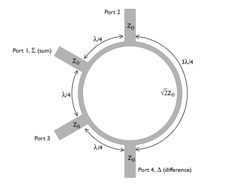
Figure 1: The geometry of rat-race coupler consists of four ports and a ring strip.
Model Definition
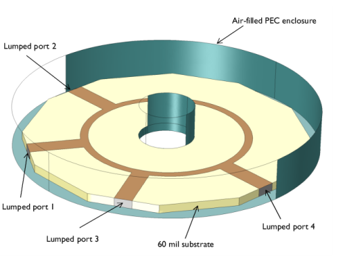
The form of the rat race coupler is shown schematically in Figure 1. The layout design is based upon Ref. 1, and is tuned to operate at 3 GHz. The design is realized as microstrip lines patterned onto a 0.060 inch dielectric substrate. The microstrip lines are modeled as perfect electric conductor (PEC) surfaces, and another PEC surface on the bottom of the dielectric substrate acts as a ground plane. The entire modeling domain is bounded by PEC boundaries that represent the device packaging. The four ports are modeled as small rectangular faces that bridge the gap between the PEC face that represents the ground plane, and the PEC faces the represent the microstrip line at each port.
Figure 2: The model of the rat-race coupler. Some exterior faces are removed for visualization.
The model is shown in Figure 2. A small air domain bounded by PEC surface around the device is also modeled. The PEC enclosure representing a metallic housing works as a cylindrical cavity. A metallic cylindrical post in the middle of the cavity is added to remove possible cavity resonances in the simulation frequency sweep range. The model is meshed using a tetrahedral mesh. A good rule of thumb is to use approximately five elements per wavelength in each material.
Results and Discussion
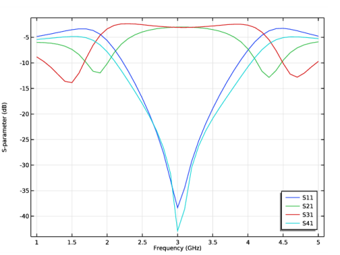
There are two paths from a source port to an observation port. The response at the observation port can be estimated from the difference between two paths. Figure 3 shows the computed S-parameters when the port 1 is excited. At a frequency of 3 GHz, the signal is evenly split between the two output ports (lumped port 2 and 3) with a very small amount of losses. The input signal is barely coupled to the isolation port (lumped port 4) where S41 is less than -30 dB at 3 GHz.
Figure 3: The frequency response of the branch line coupler shows good input matching (S11) and isolation (S41) around 3 GHz. The coupled signal at two output ports (S21 and S31) is about -3 dB at 3 GHz.
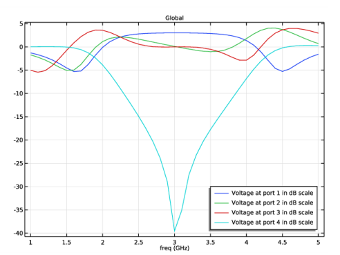
Next, the port 2 and 3 are excited evenly at the same time and the voltages at the port 1 (sum port) and port 4 (difference port) are observed. At a frequency of 3 GHz, the voltage at the port 1 is 3 dB higher than the voltage at each input port and almost zero response is shown at the port 4 where two input signals are canceled out. The sum and difference port responses are plotted in Figure 4.
Figure 4: The rat race coupler works as a power combiner, too. The responses at the sum and difference ports at 3 GHz are as expected.
References
1. D.M. Pozar, Microwave Engineering, John Wiley & Sons, 1998.
2. R.E. Collin, Foundation of Microwave Engineering, McGraw-Hill, 1992.
Application Library path: RF_Module/Couplers_and_Power_Dividers/rat_race_coupler
Modeling Instructions
From the File menu, choose New.
New
In the New window, click  Model Wizard.
Model Wizard
1
In the Model Wizard window, click  3D.
2
In the Select Physics tree, select Radio Frequency>Electromagnetic Waves, Frequency Domain (emw).
3
Click Add.
4
Click  Study.
5
In the Select Study tree, select General Studies>Frequency Domain.
6
Study 1
Step 1: Frequency Domain
1
In the Model Builder window, under Study 1 click Step 1: Frequency Domain.
2
In the Settings window for Frequency Domain, locate the Study Settings section.
3
Click  Range.
4
In the Range dialog box, type 1[GHz] in the Start text field.
5
In the Stop text field, type 5[GHz].
6
In the Step text field, type 100[MHz].
7
Click Replace.
Global Definitions
Parameters 1
1
In the Model Builder window, under Global Definitions click Parameters 1.
2
In the Settings window for Parameters, locate the Parameters section.
3
Click  Load from File.
4
Here, mil refers to the unit milliinch.
Geometry 1
Click the  Wireframe Rendering button in the Graphics toolbar.
First, create two cylinders for the metallic housing.
Cylinder 1 (cyl1)
1
In the Geometry toolbar, click  Cylinder.
2
In the Settings window for Cylinder, locate the Size and Shape section.
3
In the Radius text field, type r_subs*1.1.
4
In the Height text field, type d_subs*5.
Cylinder 2 (cyl2)
1
In the Geometry toolbar, click  Cylinder.
2
In the Settings window for Cylinder, locate the Size and Shape section.
3
In the Radius text field, type 0.005.
4
In the Height text field, type d_subs*5.
Add a work plane for the coupler layout.
Work Plane 1 (wp1)
1
In the Geometry toolbar, click  Work Plane.
Create two circles and subtract one from another for the ring strip.
2
In the Settings window for Work Plane, click  Show Work Plane.
Work Plane 1 (wp1)>Plane Geometry
In the Model Builder window, click Plane Geometry.
Work Plane 1 (wp1)>Circle 1 (c1)
1
In the Work Plane toolbar, click  Circle.
2
Click the  Zoom Extents button in the Graphics toolbar.
3
In the Settings window for Circle, locate the Size and Shape section.
4
In the Radius text field, type r_ring-w_ring/2.
Work Plane 1 (wp1)>Circle 2 (c2)
1
In the Work Plane toolbar, click  Circle.
2
In the Settings window for Circle, locate the Size and Shape section.
3
In the Radius text field, type r_ring+w_ring/2.
Work Plane 1 (wp1)>Difference 1 (dif1)
1
In the Work Plane toolbar, click  Booleans and Partitions and choose Difference.
2
3
In the Settings window for Difference, locate the Difference section.
4
Find the Objects to subtract subsection. Select the  Activate Selection toggle button.
5
Add a rectangle for the feed line and generate the four feed lines by rotating the rectangle. Use the rotation angle range to create multiple objects.
Work Plane 1 (wp1)>Rectangle 1 (r1)
1
In the Work Plane toolbar, click  Rectangle.
2
In the Settings window for Rectangle, locate the Size and Shape section.
3
In the Width text field, type w_line.
4
In the Height text field, type l_line.
5
Locate the Position section. In the xw text field, type -w_line/2.
6
In the yw text field, type r_subs-l_line.
Work Plane 1 (wp1)>Rotate 1 (rot1)
1
In the Work Plane toolbar, click  Transforms and choose Rotate.
2
3
In the Settings window for Rotate, locate the Rotation section.
4
Click  Range.
5
In the Range dialog box, type 0 in the Start text field.
6
In the Stop text field, type 180.
7
In the Step text field, type 60.
8
Click Replace.
Create a union of all 2D objects on the work plane to remove the unnecessary interior boundaries.
Work Plane 1 (wp1)>Union 1 (uni1)
1
In the Work Plane toolbar, click  Booleans and Partitions and choose Union.
2
Click in the Graphics window and then press Ctrl+A to select all objects.
3
In the Settings window for Union, locate the Union section.
4
Clear the Keep interior boundaries check box.
5
Click  Build Selected.
Add a polygon for the substrate. This polygon covers only about 1/6 of the substrate area.
Work Plane 1 (wp1)>Polygon 1 (pol1)
1
In the Work Plane toolbar, click  Polygon.
2
Click the  Zoom Extents button in the Graphics toolbar.
3
In the Settings window for Polygon, locate the Coordinates section.
4
5
Click  Build Selected.
Complete the substrate layout by rotating the polygon.
Work Plane 1 (wp1)>Rotate 2 (rot2)
1
In the Work Plane toolbar, click  Transforms and choose Rotate.
2
3
In the Settings window for Rotate, locate the Rotation section.
4
Click  Range.
5
In the Range dialog box, type 0 in the Start text field.
6
In the Stop text field, type 300.
7
In the Step text field, type 60.
8
Click Replace.
Create a union of the polygon pieces to remove the unnecessary interior boundaries.
Work Plane 1 (wp1)>Union 2 (uni2)
1
In the Work Plane toolbar, click  Booleans and Partitions and choose Union.
2
Select the objects rot2(1), rot2(2), rot2(3), rot2(4), rot2(5), and rot2(6) only.
3
In the Settings window for Union, locate the Union section.
4
Clear the Keep interior boundaries check box.
5
Click  Build Selected.
This is the rat race coupler layout on the xy-plane.
Turn the coupler layout into a 3D structure by extruding the layout.
Extrude 1 (ext1)
1
In the Model Builder window, under Component 1 (comp1)>Geometry 1 right-click Work Plane 1 (wp1) and choose Extrude.
2
In the Settings window for Extrude, click  Build All Objects.
3
Locate the Distances section. In the table, enter the following settings:
4
Click  Build All Objects.
Definitions
Create a set of selections for use while setting up the physics. First, create a selection for the substrate.
Substrate
1
In the Definitions toolbar, click  Explicit.
2
In the Settings window for Explicit, type Substrate in the Label text field.
3
Next, add a selection for the microstrip line.
Microstrip line
1
In the Definitions toolbar, click  Explicit.
2
In the Settings window for Explicit, type Microstrip line in the Label text field.
3
Locate the Input Entities section. From the Geometric entity level list, choose Boundary.
4
Add a selection for the cylindrical post in the cavity. This domain is not a part of the modeling domain.
Post
1
In the Definitions toolbar, click  Explicit.
2
In the Settings window for Explicit, type Post in the Label text field.
3
Add a selection for the modeling domain. This is the complement of the cylindrical post domain.
Model space
1
In the Definitions toolbar, click  Complement.
2
In the Settings window for Complement, type Model space in the Label text field.
3
Locate the Input Entities section. Under Selections to invert, click  Add.
4
In the Add dialog box, select Post in the Selections to invert list.
5
View 1
Hide some boundaries to get a better view of the interior parts when setting up the physics and reviewing the mesh.
Hide for Physics 1
1
In the Model Builder window, right-click View 1 and choose Hide for Physics.
2
In the Settings window for Hide for Physics, locate the Geometric Entity Selection section.
3
From the Geometric entity level list, choose Boundary.
4
Electromagnetic Waves, Frequency Domain (emw)
Now set up the physics.
1
In the Model Builder window, under Component 1 (comp1) click Electromagnetic Waves, Frequency Domain (emw).
2
In the Settings window for Electromagnetic Waves, Frequency Domain, locate the Domain Selection section.
3
From the Selection list, choose Model space.
The default boundary condition is Perfect electric conductor, which applies to all exterior boundaries. Assign Perfect electric conductor on the interior boundary on the microstrip lines.
Perfect Electric Conductor 2
1
In the Physics toolbar, click  Boundaries and choose Perfect Electric Conductor.
2
In the Settings window for Perfect Electric Conductor, locate the Boundary Selection section.
3
From the Selection list, choose Microstrip line.
Set four ports as shown in Figure 2.
Lumped Port 1
1
In the Physics toolbar, click  Boundaries and choose Lumped Port.
2
For the first port, wave excitation is on by default.
Lumped Port 2
1
In the Physics toolbar, click  Boundaries and choose Lumped Port.
2
Lumped Port 3
1
In the Physics toolbar, click  Boundaries and choose Lumped Port.
2
Lumped Port 4
1
In the Physics toolbar, click  Boundaries and choose Lumped Port.
2
Materials
Next, assign material properties to the model. Begin by specifying air for all domains.
Add Material
1
In the Home toolbar, click  Add Material to open the Add Material window.
2
Go to the Add Material window.
3
4
Click Add to Component in the window toolbar.
5
In the Home toolbar, click  Add Material to close the Add Material window.
Materials
Air (mat1)
Override the substrate with the dielectric material of εr = 3.38.
Substrate
1
In the Model Builder window, right-click Materials and choose Blank Material.
2
In the Settings window for Material, type Substrate in the Label text field.
3
Locate the Geometric Entity Selection section. From the Selection list, choose Substrate.
4
Locate the Material Contents section. In the table, enter the following settings:
Mesh 1
In the Model Builder window, under Component 1 (comp1) right-click Mesh 1 and choose Build All.
Study 1
In the Home toolbar, click  Compute.
Results
Electric Field (emw)
Begin the results analysis and visualization by modifying the first default plot to show the E-field norm on the bottom of the substrate at 3 GHz.
1
In the Settings window for 3D Plot Group, locate the Data section.
2
From the Parameter value (freq (GHz)) list, choose 3.
Multislice
1
In the Model Builder window, expand the Electric Field (emw) node, then click Multislice.
2
In the Settings window for Multislice, locate the Multiplane Data section.
3
Find the X-planes subsection. In the Planes text field, type 0.
4
Find the Y-planes subsection. In the Planes text field, type 0.
5
Find the Z-planes subsection. From the Entry method list, choose Coordinates.
6
In the Coordinates text field, type 0.
7
In the Electric Field (emw) toolbar, click  Plot.
The input power is evenly split between the two output ports.
S-parameter (emw)
1
In the Model Builder window, click S-parameter (emw).
2
In the Settings window for 1D Plot Group, locate the Legend section.
3
From the Position list, choose Lower right.
Compare the resulting plot with that shown in Figure 3.
Next, change some port settings to run the device as a power combiner and see the performance at the sum and difference ports.
Smith Plot (emw)
Electromagnetic Waves, Frequency Domain (emw)
Lumped Port 1
1
In the Model Builder window, under Component 1 (comp1)>Electromagnetic Waves, Frequency Domain (emw) click Lumped Port 1.
2
In the Settings window for Lumped Port, locate the Lumped Port Properties section.
3
From the Wave excitation at this port list, choose Off.
Lumped Port 2
1
In the Model Builder window, click Lumped Port 2.
2
In the Settings window for Lumped Port, locate the Lumped Port Properties section.
3
From the Wave excitation at this port list, choose On.
Lumped Port 3
1
In the Model Builder window, click Lumped Port 3.
2
In the Settings window for Lumped Port, locate the Lumped Port Properties section.
3
From the Wave excitation at this port list, choose On.
Add a new study for the coupler (power divider) case in order to keep the result from the previous computation.
Add Study
1
In the Home toolbar, click  Add Study to open the Add Study window.
2
Go to the Add Study window.
3
Find the Studies subsection. In the Select Study tree, select General Studies>Frequency Domain.
4
Click Add Study in the window toolbar.
5
In the Home toolbar, click  Add Study to close the Add Study window.
Study 2
Step 1: Frequency Domain
1
In the Settings window for Frequency Domain, locate the Study Settings section.
2
Click  Range.
3
In the Range dialog box, type 1[GHz] in the Start text field.
4
In the Stop text field, type 5[GHz].
5
In the Step text field, type 100[MHz].
6
Click Replace.
7
In the Model Builder window, click Study 2.
8
In the Settings window for Study, locate the Study Settings section.
9
Clear the Generate default plots check box.
10
In the Home toolbar, click  Compute.
Results
1D Plot Group 4
1
In the Home toolbar, click  Add Plot Group and choose 1D Plot Group.
2
In the Settings window for 1D Plot Group, locate the Data section.
3
From the Dataset list, choose Study 2/Solution 2 (sol2).
4
Locate the Legend section. From the Position list, choose Lower right.
Global 1
1
Right-click 1D Plot Group 4 and choose Global.
2
In the Settings window for Global, locate the y-Axis Data section.
3
4
In the 1D Plot Group 4 toolbar, click  Plot.
Compare the resulting plot with that shown in Figure 4.