Finding the Impedance of a Parallel-Wire Transmission Line

A parallel-wire transmission line is composed of two conducting wires in a dielectric such as air. The fields around such a transmission line are not directly confined by the conductors but extend to infinity, although they drop off rapidly away from the wires. This example demonstrates how to compute the fields and impedance of such an unshielded transmission line and compares the results to the analytic solution.

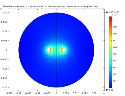
Figure 1: A parallel-wire transmission line. The electric field strength is plotted in color while arrows show the magnetic field.

Model Definition

Because a parallel-wire transmission line operates in TEM mode?with the electric and magnetic fields normal to the direction of propagation along the cable?modeling a 2D cross section suffices to compute the fields and the impedance. For this example, assume perfect conductors and a lossless air region. The wires, of radius is 1 mm, are separated by a center-to-center distance of 8 mm.

Because the structure is open, the fields extend infinitely far away from the wires. However, they drop off quickly in magnitude. This raises the question about what boundary condition to use on the air domain’s outer boundary. The surrounding dielectric medium can be thought of as a perfect insulator, as opposed to the wires, which are modeled as perfect conductors. Thus, the model uses a perfect magnetic conductor (PMC) boundary condition, because this condition is, in a sense, the opposite of the perfect electric conductor (PEC) boundary condition. However, it must be placed some distance away from the wires or else it would artificially confine the fields. In this example, the air domain’s radius is chosen to be five times the distance from its center to the center of each wire. Increasing this radius would give a more accurate solution at the cost of a more memory-intensive computation.

Figure 2: The impedance of a parallel-wire transmission line can be found from the voltage, V, and current, I, which are computed via line integrals as shown.

The characteristic impedance, Z0 = V/I, of a transmission line relates the voltage to the current. Although the model does not involve computing the potential field, the voltage of the TEM waveguide can be evaluated as a line integral of the electric field between the conductors:

(1)

The voltage and current in the direction out of the plane are positive for integration paths oriented as in Figure 2.

The value of Z0 obtained in this way, should be compared with the analytic result

Here ra is the wire radius and rd is the center-to-center distance between the wires.

Results and Discussion

Figure 3 is a combined plot of the electric field magnitude and the magnetic field visualized as an arrow plot.

Figure 3: Electric field magnitude (surface) and magnetic field (arrows) around the two parallel wires.

The impedance computed with the default mesh is Z0 = 255.8 Ω. As the radius of the dielectric domain is increased, the numerical solution will approach the analytic value of 247.4 Ω.

Notes About the COMSOL Implementation

Solve this example using a Mode Analysis study and the default frequency, f = 1 GHz.

RF_Module/Verification_Examples/parallel_wires_impedance

Modeling Instructions

From the menu, choose .

New

In the window, click

Model Wizard

In the window, click

In the tree, select .

Click .

Click

In the tree, select .

Click

Global Definitions

Parameters 1

In the window, under click .

In the window for , locate the section.

In the table, enter the following settings:


Name	Expression	Value	Description
r_a	1[mm]	0.001 m	Wire radius
r_d	4[mm]	0.004 m	Center-to-center distance between wires
r_air	5*r_d	0.02 m	Air-domain radius
Z0_analytic	(Z0_const/pi)*log(r_d/r_a+sqrt((r_d/r_a)^2-1))	247.44 Ω	Characteristic impedance, analytic

Here, Z0_const is a predefined COMSOL constant for the characteristic impedance of vacuum, Z0 = sqrt(μ0/ε0). From the Value column you can read off the value Z0,analytic = 247 Ω. Note also that the logarithm in the definition for Z0_analytic is an equivalent way of writing acosh(r_d/r_a).

Geometry 1

First, create a circle for the air domain.

Circle 1 (c1)

In the toolbar, click

In the window for , locate the section.

In the text field, type r_air.

Click

Add a circle for one wire.

Circle 2 (c2)

In the toolbar, click

In the window for , locate the section.

In the text field, type r_a.

Locate the section. In the text field, type r_d.

Click

Then, generate the other wire by mirroring the above one.

Mirror 1 (mir1)

In the toolbar, click

and choose .

Select the object only.

In the window for , locate the section.

Select the check box.

Click

Difference 1 (dif1)

In the toolbar, click

and choose .

Select the object only.

In the window for , locate the section.

Find the subsection. Select the

toggle button.

Select the objects and only.

Click

Create a line for computing the voltage as a line integral of the electric field.

Line Segment 1 (ls1)

In the toolbar, click

and choose .

In the window for , locate the section.

From the list, choose .

Locate the section. From the list, choose .

Locate the section. In the text field, type -r_d+r_a.

Locate the section. In the text field, type r_d-r_a.

Add a line, a part of the closed contour for computing the current as a line integral of the magnetic field.

Line Segment 2 (ls2)

In the toolbar, click

and choose .

In the window for , locate the section.

From the list, choose .

Locate the section. From the list, choose .

Locate the section. In the text field, type -r_air.

Locate the section. In the text field, type r_air.

Click

The model layout describes two parallel wires in the air.

Definitions

Add a variable for the characteristic impedance computed as the voltage between the wires divided by the current through the wires. Define two nonlocal integration couplings for computing the voltage and the current.

Integration 1 (intop1)

In the toolbar, click

and choose .

In the window for , type int_E in the text field.

Locate the section. From the list, choose .

Select Boundaries 1 and 4 only.

Integration 2 (intop2)

In the toolbar, click

and choose .

In the window for , type int_H in the text field.

Locate the section. From the list, choose .

Select Boundaries 2, 3, 11, and 12 only.

Because of the PMC boundary condition, there is no tangential H-field on the outermost boundaries. It is therefore possible to omit Boundaries 11 and 12 when computing the current even though the model includes those boundaries.

Study 1

Step 1: Mode Analysis

In the window, under click .

In the window for , locate the section.

Select the check box.

In the associated text field, type 1.

Definitions

Variables 1

In the toolbar, click

In the window for , locate the section.

In the table, enter the following settings:


Name	Expression	Unit	Description
V	int_E(-emw.Ext1x-emw.Eyt1y)	V	Voltage
I	-int_H(emw.Hxt1x+emw.Hyt1y)	A	Current
Z_model	V/I	Ω	Characteristic impedance

Here, t1x and t1y are the tangential vector components along the integration boundaries (1 refers to the boundary dimension). The emw. prefix gives the correct physics-interface scope for the electric and magnetic field vector components.

Electromagnetic Waves, Frequency Domain (emw)

Now set up the physics. The default boundary condition is perfect electric conductor. Override the outermost boundaries with a perfect magnetic conductor condition to create a virtually infinite modeling space.

Perfect Magnetic Conductor 1

In the window, under right-click and choose .

Select Boundaries 5, 6, 11, and 12 only.

Materials

Next, assign a material to the modeling domain.

Add Material

In the toolbar, click

to open the window.

Go to the window.

In the tree, select .

Click in the window toolbar.

In the toolbar, click

to close the window.

Mesh 1

Use the default mesh.

In the window, under click .

In the window for , locate the section.

In the table, clear the check box for .

Click

Study 1

In the toolbar, click

Results

Electric Field (emw)

The default plot shows the distribution of the norm of the electric field. Add an arrow plot of the magnetic field.

Arrow Surface 1

Right-click and choose .

In the window for , locate the section.

Find the subsection. In the text field, type 30.

In the toolbar, click

Locate the section. From the list, choose .

Select the check box.

In the associated text field, type 1.2e-4.

You can use the slider to adjust the arrow-length scale factor.

Compare the resulting plot with that shown in Figure 3.

Add an arrow plot along the boundaries to see the orientation of tangent vector field.

Arrow Line 1

Right-click and choose .

In the window for , click in the upper-right corner of the section. From the menu, choose .

In the toolbar, click

Locate the section. In the text field, type 100.

In the toolbar, click

A comparison with Equation 1 reveals that the line integral for the voltage computes the potential difference V2 - V1. When computing the line integral for the current, the clockwise orientation of the integration contour would mean that a positive current is directed in the negative z direction, that is, into the modeling plane. The minus sign added in the definition of I reverses this direction.

Finish by computing the characteristic impedance.

Global Evaluation 1

In the toolbar, click

In the window for , locate the section.

In the table, enter the following settings:


Expression	Unit	Description
Z_model	Ω	Characteristic impedance

Click

Table

Go to the window.

The value shown in the Table window should be close to 255.8Ω. You can get closer to the analytic value 247.4Ω by increasing the air-domain radius. For example, changing the definition of r_air to 10*r_d under Global Definitions>Parameters and re-solving the model gives the value 248.9Ω.