PDF

Parabolic Reflector Antenna
Introduction
A large reflector can be modeled easily with the 2D axisymmetric formulation. In this example, the radius of the reflector is greater than 20 wavelengths and the reflector is illuminated by an axial feed circular horn antenna. The simulated far-field shows a high-gain sharp beam pattern.
Figure 1: This is a 3D visualization of the parabolic reflector antenna that is solved using the 2D axisymmetric formulation.
Model Definition
Since the axial feed circular horn and parabolic reflector antenna are solids of revolution, the antenna can be simulated using the 2D axisymmetric formulation of the electromagnetic wave equation (Figure 1). This approach overcomes a general difficulty when optimizing a reflector antenna: due to its very large size in terms of wavelength, the 3D calculation is computationally intensive.
In this example, all metal surfaces are modeled as perfect electric conductors (PECs) and all domains are filled with air.
The radius of the circular horn feed waveguide is 0.01 m and the cutoff frequency of the TE11 mode is approximately 8.8 GHz. The operating frequency of the antenna should be higher than the cutoff frequency. The horn aperture radius is 0.03 m and the overall horn length is 0.06 m. A slit-conditioned circular port is assigned on the end of the waveguide to excite the antenna with the TE1m mode. The azimuthal mode number, m, is defined from the Electromagnetic Waves, Frequency Domain interface. In this example, m 1.
The reflector is built using a 53 degree sector of a circle with a radius of 0.85 m. The reflector body is removed from the model domain and, consequently, the PEC is automatically applied to its boundary. The model domain is enclosed by perfectly matched layers (PMLs). The PMLs are thicker than that of other antenna examples in the Application Libraries since high gain and stronger propagation are expected from the reflector.
A Free Triangular mesh is used for the antenna and air domains. The maximum element size is one-fifth of the wavelength at the simulation frequency. A mapped mesh with 10 layers is used for the PMLs.
Results and Discussion
In Figure 2, the norm of the electric field is plotted in decibels with arrows indicating the direction and relative magnitude of power flow. The field from the horn antenna is reflected by the parabola and propagates in the +z direction, confined near the axis of rotation.
The 3D far-field radiation pattern is plotted with a visualization of the antenna body in Figure 3. The low gain radiation from the axial feed horn results in a very high gain pattern created by the reflector.
The far-field radiation pattern in Figure 3 is just a simple body of revolution of the 2D plot data that is useful to measure quickly the maximum gain and review the overall shape of the pattern. The effective 3D far-field radiation pattern of the antenna excited by TE11 mode can be estimated using the predefined postprocessing function, normdB3DEfar_TE11(angle), that is shown in Figure 4.
Figure 2: The norm of the electric field is plotted in decibels. The field from the horn antenna is reflected by the parabola and propagates in the +z direction.
Figure 3: The very sharp 3D far-field radiation pattern is visualized over the axial feed circular horn and parabolic reflector.
Figure 4: Effective 3D far-field radiation pattern plotted in 80 dB dynamic range using far-far field function normdB3DEfar_TE11(angle).
Application Library path: RF_Module/Antennas/parabolic_reflector
Modeling Instructions
From the File menu, choose New.
New
In the New window, click  Model Wizard.
Model Wizard
1
In the Model Wizard window, click  2D Axisymmetric.
2
In the Select Physics tree, select Radio Frequency>Electromagnetic Waves, Frequency Domain (emw).
3
Click Add.
4
Click  Study.
5
In the Select Study tree, select General Studies>Frequency Domain.
6
Global Definitions
Parameters 1
1
In the Model Builder window, under Global Definitions click Parameters 1.
2
In the Settings window for Parameters, locate the Parameters section.
3
Here, c_const is a predefined COMSOL constant for the speed of light in vacuum.
Study 1
Step 1: Frequency Domain
1
In the Model Builder window, under Study 1 click Step 1: Frequency Domain.
2
In the Settings window for Frequency Domain, locate the Study Settings section.
3
In the Frequencies text field, type f0.
Geometry 1
Rectangle 1 (r1)
1
In the Geometry toolbar, click  Rectangle.
2
In the Settings window for Rectangle, locate the Size and Shape section.
3
In the Width text field, type r1.
4
In the Height text field, type 0.06.
Polygon 1 (pol1)
1
In the Geometry toolbar, click  Polygon.
2
In the Settings window for Polygon, locate the Coordinates section.
3
4
Click  Build Selected.
Circle 1 (c1)
1
In the Geometry toolbar, click  Circle.
2
In the Settings window for Circle, locate the Size and Shape section.
3
In the Radius text field, type 0.9.
4
In the Sector angle text field, type 180.
5
Locate the Rotation Angle section. In the Rotation text field, type 270.
6
Click to expand the Layers section. In the table, enter the following settings:
7
Click  Build Selected.
8
Click the  Zoom Extents button in the Graphics toolbar.
Circle 2 (c2)
1
In the Geometry toolbar, click  Circle.
2
In the Settings window for Circle, locate the Size and Shape section.
3
In the Radius text field, type r0.
4
In the Sector angle text field, type 53.
5
Locate the Position section. In the z text field, type r0-0.365.
6
Locate the Rotation Angle section. In the Rotation text field, type 270.
7
Locate the Layers section. In the table, enter the following settings:
Delete Entities 1 (del1)
1
In the Model Builder window, right-click Geometry 1 and choose Delete Entities.
2
On the object c2, select Boundary 1 only.
3
In the Settings window for Delete Entities, click  Build All Objects.
The finished geometry should look like this.
Definitions
Perfectly Matched Layer 1 (pml1)
1
In the Definitions toolbar, click  Perfectly Matched Layer.
2
Electromagnetic Waves, Frequency Domain (emw)
1
In the Model Builder window, under Component 1 (comp1) click Electromagnetic Waves, Frequency Domain (emw).
2
The reflector body is removed from the model domain and, consequently, the PEC is automatically applied to its boundary.
3
In the Settings window for Electromagnetic Waves, Frequency Domain, locate the Out-of-Plane Wave Number section.
4
In the m text field, type 1.
Perfect Electric Conductor 2
1
In the Physics toolbar, click  Boundaries and choose Perfect Electric Conductor.
2
Port 1
1
In the Physics toolbar, click  Boundaries and choose Port.
2
3
In the Settings window for Port, locate the Port Properties section.
4
From the Type of port list, choose Circular.
For the first port, wave excitation is on by default.
5
Select the Activate slit condition on interior port check box.
6
Click Toggle Power Flow Direction.
Scattering Boundary Condition 1
1
In the Physics toolbar, click  Boundaries and choose Scattering Boundary Condition.
2
Far-Field Domain 1
In the Physics toolbar, click  Domains and choose Far-Field Domain.
Materials
Material 1 (mat1)
1
In the Model Builder window, under Component 1 (comp1) right-click Materials and choose Blank Material.
2
In the Settings window for Material, locate the Material Contents section.
3
Mesh 1
1
In the Model Builder window, under Component 1 (comp1) right-click Mesh 1 and choose Build All.
2
Click the  Zoom In button in the Graphics toolbar, a couple of times to get a better view of the meshed structure.
Study 1
In the Home toolbar, click  Compute.
Results
Surface
1
In the Model Builder window, expand the Electric Field (emw) node, then click Surface.
2
In the Settings window for Surface, locate the Expression section.
3
In the Expression text field, type 20*log10(emw.normE).
4
In the Electric Field (emw) toolbar, click  Plot.
Arrow Surface 1
1
In the Model Builder window, right-click Electric Field (emw) and choose Arrow Surface.
2
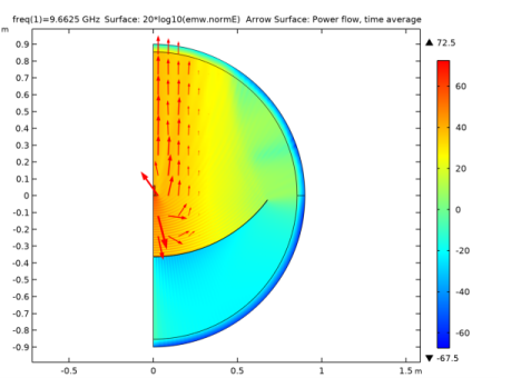
In the Settings window for Arrow Surface, click Replace Expression in the upper-right corner of the Expression section. From the menu, choose Component 1 (comp1)>Electromagnetic Waves, Frequency Domain>Energy and power>emw.Poavr,emw.Poavz - Power flow, time average.
3
Locate the Coloring and Style section. From the Arrow length list, choose Logarithmic.
4
Select the Scale factor check box.
5
6
In the Electric Field (emw) toolbar, click  Plot.
7
Click the  Zoom Extents button in the Graphics toolbar.
Compare with the plot in Figure 2.
Radiation Pattern 1
Increase the resolution of the far field polar plot.
1
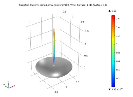
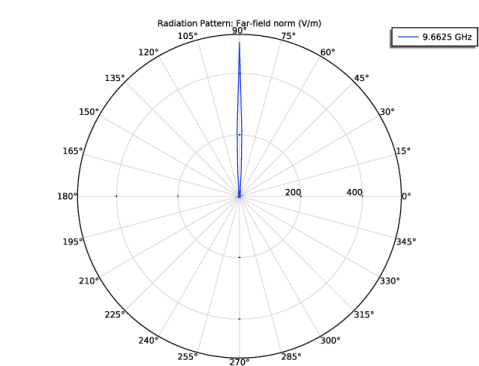
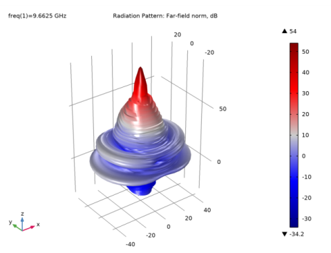
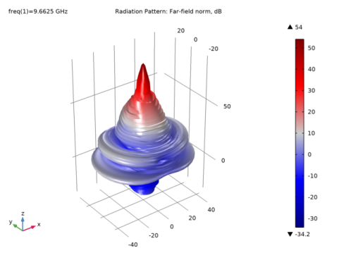
In the Model Builder window, expand the Results>2D Far Field (emw) node, then click Radiation Pattern 1.
2
In the Settings window for Radiation Pattern, locate the Evaluation section.
3
Find the Angles subsection. In the Number of angles text field, type 180.
4
Find the Reference direction subsection. In the x text field, type -1.
5
In the z text field, type 0.
6
In the 2D Far Field (emw) toolbar, click  Plot.
Study 1/Solution 1 (2) (sol1)
In the Results toolbar, click  More Datasets and choose Solution.
Selection
1
In the Results toolbar, click  Attributes and choose Selection.
2
In the Settings window for Selection, locate the Geometric Entity Selection section.
3
From the Geometric entity level list, choose Domain.
4
Revolution 2D Feed horn
1
In the Results toolbar, click  More Datasets and choose Revolution 2D.
2
In the Settings window for Revolution 2D, type Revolution 2D Feed horn in the Label text field.
3
Locate the Data section. From the Dataset list, choose Study 1/Solution 1 (2) (sol1).
Study 1/Solution 1 (3) (sol1)
In the Results toolbar, click  More Datasets and choose Solution.
Selection
1
In the Results toolbar, click  Attributes and choose Selection.
2
In the Settings window for Selection, locate the Geometric Entity Selection section.
3
From the Geometric entity level list, choose Domain.
4
Revolution 2D Reflector
1
In the Results toolbar, click  More Datasets and choose Revolution 2D.
2
In the Settings window for Revolution 2D, type Revolution 2D Reflector in the Label text field.
3
Locate the Data section. From the Dataset list, choose Study 1/Solution 1 (3) (sol1).
Surface 1
1
In the Model Builder window, right-click 3D Far Field (emw) and choose Surface.
2
In the Settings window for Surface, locate the Data section.
3
From the Dataset list, choose Revolution 2D Feed horn.
4
Locate the Expression section. In the Expression text field, type 1.
5
Locate the Coloring and Style section. From the Coloring list, choose Uniform.
6
From the Color list, choose Yellow.
Surface 2
1
Right-click 3D Far Field (emw) and choose Surface.
2
In the Settings window for Surface, locate the Data section.
3
From the Dataset list, choose Revolution 2D Reflector.
4
Locate the Expression section. In the Expression text field, type 1.
5
Locate the Coloring and Style section. From the Coloring list, choose Uniform.
6
From the Color list, choose Gray.
Radiation Pattern 1
1
In the Model Builder window, click Radiation Pattern 1.
2
In the Settings window for Radiation Pattern, locate the Expression section.
3
In the Expression text field, type comp1.emw.normEfar/300.
4
In the 3D Far Field (emw) toolbar, click  Plot.
Table
1
Go to the Table window.
2
Click the  Zoom Extents button in the Graphics toolbar.
The plotted figure describes the axial feed circular horn and parabolic reflector as well as the 3D far-field pattern as shown in Figure 3.
The 3D far-field radiation pattern plotted by default is just a simple body of revolution of the 2D plot that is useful to measure quickly the maximum gain. Using the predefined postprocessing function, it is possible to estimate an effective 3D far-field radiation pattern of the antenna that is excited by the dominant mode of the 3D model of a circular waveguide, TE11 mode.
Results
3D Plot Group 4
1
In the Home toolbar, click  Add Plot Group and choose 3D Plot Group.
2
In the Settings window for 3D Plot Group, locate the Data section.
3
From the Dataset list, choose None.
4
Locate the Color Legend section. Select the Show maximum and minimum values check box.
Radiation Pattern 1
1
In the 3D Plot Group 4 toolbar, click  More Plots and choose Radiation Pattern.
2
In the Settings window for Radiation Pattern, locate the Data section.
3
From the Dataset list, choose Study 1/Solution 1 (1) (sol1).
4
Locate the Expression section. In the Expression text field, type emw.normdB3DEfar_TE11(angle).
5
Locate the Evaluation section. Find the Angles subsection. In the Number of elevation angles text field, type 180.
6
In the Number of azimuth angles text field, type 45.
7
In the Azimuthal angle variable text field, type angle.
The far-field function contains an argument, which is given the name angle by default. For the azimuthal angle variable field in the Evaluation section, enter angle to match the function argument. Note that the name can be chosen freely as long as the function argument matches the azimuth angle variable specified in the Evaluation section. This plot would take up to several minutes.
8
Locate the Coloring and Style section. From the Color table list, choose Wave.
9
In the 3D Plot Group 4 toolbar, click  Plot.
Compare the plot with Figure 4.