PDF

Coaxial to Waveguide Coupling
Introduction
Feeding a waveguide from a coaxial cable is a straightforward way to get electromagnetic waves inside the waveguide. This example shows how to compute the reflection and transmission in a coupling from a coaxial cable to a rectangular waveguide.
Model Definition
As seen in the results plot in Figure 1, the coaxial cable is attached to an opening in the bottom of the rectangular waveguide. The inner conductor of the cable continues into the waveguide in order to transmit the waves. The model is run at a frequency of 6 GHz.
The wave coming in through the coaxial cable is set up using a Port boundary condition, with a 1 W coaxial feed selected. At the passive output port, the fundamental rectangular TE10 mode is assumed. The interpretation of the port conditions is that the coaxial cable and the rectangular waveguide continue indefinitely outside the model. The model therefore isolates the properties of the coupling from the properties of any outside circuit connecting to the other end of the waveguide or the cable.
The port boundary conditions are perfectly transparent only to their own specified mode. These same modes are also used in the automatic S-parameter analysis. For these reasons, it is important that the modeled sections are long enough that any evanescent waves have almost completely died out before they reach the ports. This leaves only the propagating modes - at 6 GHz, the only supported propagating modes are the specified, fundamental modes.
An impedance boundary condition with material properties for copper is used for the coaxial conductors and the metal surfaces of the waveguide. At the considered frequency, copper is such a good conductor that a perfect electric conductor condition would be a reasonable alternative. However, the impedance condition also helps to accommodate the port boundaries, by smoothing out any numerical inconsistencies at the edges where they meet.
Results and Discussion
For cable feeds it is interesting to compare the reflected wave going back into the coaxial cable with the wave propagating in the rectangular waveguide. You can make such a comparison by evaluating the S-parameter on the coaxial port and compare it with the S-parameter on the rectangular port. The following table shows the result for a frequency of 6 GHz in dB scale:
The following plot shows the electric field distribution. The z-component is shown in the rectangular waveguide and the y-component on a vertical slice through the coaxial cable and into the waveguide. Except for just at the end of the inner coaxial conductor, the x- and y-components of the field are negligible in the waveguide. Likewise, the z-component is barely present in the coaxial cable.
Figure 1: Horizontal slice through the rectangular waveguide showing the z-component of the field, and vertical slice through the coaxial cable showing the y-component.
Application Library path: RF_Module/Transmission_Lines_and_Waveguides/coaxial_waveguide_coupling
Modeling Instructions
From the File menu, choose New.
New
In the New window, click  Model Wizard.
Model Wizard
1
In the Model Wizard window, click  3D.
2
In the Select Physics tree, select Radio Frequency>Electromagnetic Waves, Frequency Domain (emw).
3
Click Add.
4
Click  Study.
5
In the Select Study tree, select General Studies>Frequency Domain.
6
Study 1
Step 1: Frequency Domain
1
In the Model Builder window, under Study 1 click Step 1: Frequency Domain.
2
In the Settings window for Frequency Domain, locate the Study Settings section.
3
In the Frequencies text field, type 6[GHz].
Global Definitions
To help in creating the geometry, define some parameters defining its dimensions.
Parameters 1
1
In the Model Builder window, under Global Definitions click Parameters 1.
2
In the Settings window for Parameters, locate the Parameters section.
3
The width of the waveguide is taken to be twice the height.
Geometry 1
Block 1 (blk1)
1
In the Geometry toolbar, click  Block.
2
In the Settings window for Block, locate the Size and Shape section.
3
In the Width text field, type L.
4
In the Depth text field, type 2*H.
5
In the Height text field, type H.
Cylinder 1 (cyl1)
1
In the Geometry toolbar, click  Cylinder.
2
In the Settings window for Cylinder, locate the Size and Shape section.
3
In the Radius text field, type R.
4
In the Height text field, type l.
5
Locate the Position section. In the x text field, type H.
6
In the y text field, type H.
7
In the z text field, type -l.
8
Click  Build All Objects.
Cylinder 2 (cyl2)
1
In the Geometry toolbar, click  Cylinder.
2
In the Settings window for Cylinder, locate the Size and Shape section.
3
In the Radius text field, type r.
4
In the Height text field, type l+H/2.
5
Locate the Position section. In the x text field, type H.
6
In the y text field, type H.
7
In the z text field, type -l.
8
Click  Build All Objects.
As you are going to represent all conductors as boundaries, you will now create a hole in the geometry replacing the inner conductor of the coaxial cable.
9
Click the  Wireframe Rendering button in the Graphics toolbar.
Difference 1 (dif1)
1
In the Geometry toolbar, click  Booleans and Partitions and choose Difference.
2
3
Select the objects blk1 and cyl1 only.
4
In the Settings window for Difference, locate the Difference section.
5
Find the Objects to subtract subsection. Select the  Activate Selection toggle button.
Select and add the inner cylinder of the coaxial cable.
6
7
Click  Build All Objects.
Definitions
With the geometry set up, define a couple of boundary selections to allow for quick access to some commonly used boundaries.
Metal Boundaries
1
In the Definitions toolbar, click  Explicit.
2
In the Settings window for Explicit, type Metal Boundaries in the Label text field.
3
Locate the Input Entities section. From the Geometric entity level list, choose Boundary.
4
Select the All boundaries check box.
5
Remove Boundaries 8 and 21 from the selection. These are the boundaries where the wave will enter and leave your waveguide coupling.
Input Port
1
In the Definitions toolbar, click  Explicit.
2
In the Settings window for Explicit, type Input Port in the Label text field.
3
Locate the Input Entities section. From the Geometric entity level list, choose Boundary.
4
Boundary 8 is the outer face of the coaxial cable.
Output Port
1
In the Definitions toolbar, click  Explicit.
2
In the Settings window for Explicit, type Output Port in the Label text field.
3
Locate the Input Entities section. From the Geometric entity level list, choose Boundary.
4
Boundary 21 is the boundary on the far end of the rectangular waveguide section.
Add Material
1
In the Home toolbar, click  Add Material to open the Add Material window.
2
Go to the Add Material window.
3
4
Click Add to Component in the window toolbar.
Materials
Air (mat1)
Select Domain 1 only.
Dielectric
1
In the Model Builder window, right-click Materials and choose Blank Material.
2
In the Settings window for Material, type Dielectric in the Label text field.
3
4
Locate the Material Contents section. In the table, enter the following settings:
Add Material
1
Go to the Add Material window.
2
In the tree, select Built-in>Copper.
3
Click Add to Component in the window toolbar.
4
In the Home toolbar, click  Add Material to close the Add Material window.
Materials
Copper (mat3)
1
In the Settings window for Material, locate the Geometric Entity Selection section.
2
From the Geometric entity level list, choose Boundary.
3
From the Selection list, choose Metal Boundaries.
Electromagnetic Waves, Frequency Domain (emw)
Impedance Boundary Condition 1
1
In the Model Builder window, under Component 1 (comp1) right-click Electromagnetic Waves, Frequency Domain (emw) and choose Impedance Boundary Condition.
2
In the Settings window for Impedance Boundary Condition, locate the Boundary Selection section.
3
From the Selection list, choose Metal Boundaries.
Port 1
1
In the Physics toolbar, click  Boundaries and choose Port.
2
In the Settings window for Port, locate the Boundary Selection section.
3
From the Selection list, choose Input Port.
4
Locate the Port Properties section. From the Type of port list, choose Coaxial.
For the first port, wave excitation is on by default.
Port 2
1
In the Physics toolbar, click  Boundaries and choose Port.
2
In the Settings window for Port, locate the Boundary Selection section.
3
From the Selection list, choose Output Port.
4
Locate the Port Properties section. From the Type of port list, choose Rectangular.
Mesh 1
In the Model Builder window, under Component 1 (comp1) right-click Mesh 1 and choose Build All.
Study 1
In the Home toolbar, click  Compute.
Results
Multislice
1
In the Model Builder window, expand the Electric Field (emw) node, then click Multislice.
2
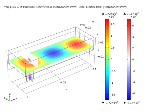
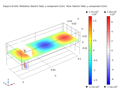
In the Settings window for Multislice, click Replace Expression in the upper-right corner of the Expression section. From the menu, choose Component 1 (comp1)>Electromagnetic Waves, Frequency Domain>Electric>Electric field - V/m>emw.Ez - Electric field, z component.
3
Locate the Multiplane Data section. Find the X-planes subsection. In the Planes text field, type 0.
4
Find the Y-planes subsection. In the Planes text field, type 0.
5
Find the Z-planes subsection. From the Entry method list, choose Coordinates.
6
In the Coordinates text field, type H/4.
7
In the Electric Field (emw) toolbar, click  Plot.
Slice 1
1
In the Model Builder window, right-click Electric Field (emw) and choose Slice.
2
In the Settings window for Slice, click Replace Expression in the upper-right corner of the Expression section. From the menu, choose Component 1 (comp1)>Electromagnetic Waves, Frequency Domain>Electric>Electric field - V/m>emw.Ey - Electric field, y component.
3
Locate the Plane Data section. From the Entry method list, choose Coordinates.
4
In the X-coordinates text field, type H.
5
Click to expand the Inherit Style section. Locate the Coloring and Style section. From the Color table list, choose WaveLight.
6
In the Electric Field (emw) toolbar, click  Plot.
In the coaxial cable, the field is largely radial, meaning the y component dominates. The other slice shows the field in the rectangular waveguide, where the z component takes over.
The port conditions automatically compute and supply the S-parameters.