Circular Waveguide Filter

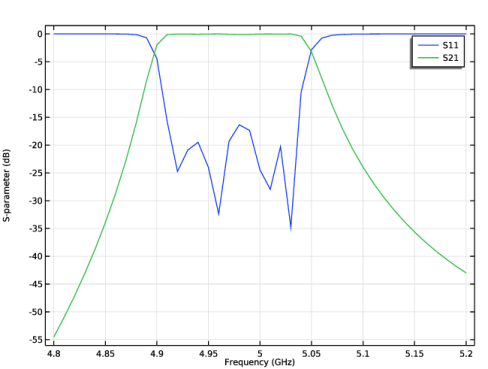
A circular waveguide filter is designed using a 2D axisymmetric model. Six annular rings added to the waveguide form circular cavities connected in series, and each cavity cutoff frequency is close to the center frequency of the filter. The computed S-parameters show a bandpass frequency response.

Figure 1: 3D visualization of the circular waveguide with irises from a 2D axisymmetric model.

Model Definition

The model consists of a C-band circular waveguide and six irises. The waveguide walls and iris parts are modeled as perfect electric conductors (PECs) and the inside of the waveguide is set to vacuum.

One end of the circular waveguide is excited with a predefined TE1 mode port boundary condition and the other end is terminated with a passive port boundary condition for the same mode. The combination of azimuthal mode index and the circular port mode index in a 2D axisymmetric model is compatible with the predefined circular port mode index of a 3D model. The TE11 mode cutoff frequency of a circular waveguide with radius of 20 mm is approximately 4.4 GHz, which is calculated by

where c0 is the speed of light, p′nm are the roots of the derivative of the Bessel functions Jn(x), m and n are the mode indices, and a is the radius of a waveguide. The value of p′11 is approximately 1.841. The operating frequency of the filter is necessarily higher than the waveguide cutoff frequency.

The center frequency of the filter is estimated by evaluating the resonance frequency of a hypothetical closed cavity formed by the waveguide and closed irises. that is, a cylindrical cavity, The resonance frequency of the cylindrical cavity is

where μr is relative permeability, εr is relative permittivity, d is the length of a cavity and l is the longitudinal cavity mode index (along the cylindrical axis). The remaining parameters are identical to those of a circular waveguide cutoff frequency. The resonance frequency at TE111 mode of the cylindrical cavity is approximately 5.05 GHz. This approximation is obtained assuming that the irises are closed, and so there is only one discrete resonance frequency where the field is nonzero. A more accurate frequency response of the filter is obtained by solving the problem with open irises.

All domains are meshed by a tetrahedral mesh with maximum element size of ten elements per wavelength so that the wave is well resolved.

Results and Discussion

The default plot shows the norm of the electric field in the waveguide. The standing wave pattern within each partitioned section of the waveguide at 4.98 GHz illustrates that this is a resonance frequency. It also demonstrates qualitatively that each partitioned section of the waveguide functions as a cavity with open ends at the irises.

Figure 2: The E-field norm shows a standing wave pattern near the center frequency of the filter. The plot illustrates that each partitioned section of the waveguide forms an open cavity.

Figure 3 shows the calculated S-parameters as a function of frequency. The passband for the filter is approximately 4.98 GHz and the insertion loss is close to 0 dB.

Figure 3: The S-parameter plot shows a bandpass frequency response. The sharp out-of-band rejection below the cutoff frequency is observed.

Notes About the COMSOL Implementation

The assumed temporal and angular dependence of all field quantities in the 2D axisymmetric formulation is ej(ωt-mφ), where ω is the angular frequency and m is the azimuthal mode number.

RF_Module/Filters/circular_waveguide_filter

Modeling Instructions

From the menu, choose .

New

In the window, click

Model Wizard

In the window, click

In the tree, select .

Click .

Click

In the tree, select .

Click

Study 1

Step 1: Frequency Domain

In the window, under click .

In the window for , locate the section.

In the text field, type range(4.8[GHz],10[MHz],5.2[GHz]).

The choices of 4.8 GHz and 5.2 GHz ensured that the parametric sweep will start above the cutoff frequency and contain the resonant frequency.

Global Definitions

Parameters 1

In the window, under click .

In the window for , locate the section.

Click

Browse to the model’s Application Libraries folder and double-click the file circular_waveguide_filter_parameters.txt.

First load the geometric parameters. Now, we will first calculate the cutoff and resonant frequency of the waveguide to choose appropriate values for the parametric sweep.

In the table, enter the following settings:


Name	Expression	Value	Description
fnml	c_const/pi/2*sqrt((1.841/r1)^2+(pi/0.06)^2)	5.0528E9 1/s	Cavity resonance frequency
fc	1.841*c_const/2/pi/r1	4.392E9 1/s	Cutoff frequency

Here, c_const is a predefined COMSOL constant for the speed of light in vacuum.

Geometry 1

Rectangle 1 (r1)

In the toolbar, click

In the window for , locate the section.

In the text field, type r1.

In the text field, type 0.4.

Locate the section. In the text field, type -0.2.

Rectangle 2 (r2)

In the toolbar, click

In the window for , locate the section.

In the text field, type ir1.

In the text field, type irth.

Locate the section. In the text field, type r1-ir1.

In the text field, type -cl3/2-cl2-cl1-irth/2.

Rectangle 3 (r3)

In the toolbar, click

In the window for , locate the section.

In the text field, type ir2.

In the text field, type irth.

Locate the section. In the text field, type r1-ir2.

In the text field, type -cl3/2-cl2-irth/2.

Rectangle 4 (r4)

In the toolbar, click

In the window for , locate the section.

In the text field, type ir3.

In the text field, type irth.

Locate the section. In the text field, type r1-ir3.

In the text field, type -cl3/2-irth/2.

Mirror 1 (mir1)

In the toolbar, click

and choose .

Select the objects , , and only.

In the window for , locate the section.

Select the check box.

Locate the section. In the text field, type 0.

In the text field, type 1.

Difference 1 (dif1)

In the toolbar, click

and choose .

Select the object only.

In the window for , locate the section.

Find the subsection. Select the

toggle button.

Select the objects , , , , , and only.

Click

The finished geometry should look like this.

Electromagnetic Waves, Frequency Domain (emw)

In the window, under click .

In the window for , locate the section.

In the m text field, type 1.

This defines the azimuthal dependency of the fields that the model is solving for.

Port 1

In the toolbar, click

and choose .

Select Boundary 2 only.

In the window for , locate the section.

From the list, choose .

For the first port, wave excitation is by default.

Port 2

In the toolbar, click

and choose .

Select Boundary 3 only.

In the window for , locate the section.

From the list, choose .

Materials

Material 1 (mat1)

In the window, under right-click and choose .

In the window for , locate the section.

In the table, enter the following settings:


Property	Variable	Value	Unit	Property group
Relative permittivity	epsilonr_iso ; epsilonrii = epsilonr_iso, epsilonrij = 0	1	1	Basic
Relative permeability	mur_iso ; murii = mur_iso, murij = 0	1	1	Basic
Electrical conductivity	sigma_iso ; sigmaii = sigma_iso, sigmaij = 0	0	S/m	Basic

Mesh 1

In the window, under right-click and choose .

Study 1

In the toolbar, click

Results

Electric Field (emw)

In the window for , locate the section.

From the list, choose .

In the toolbar, click

S-parameter (emw)

This reproduces Figure 3.