Car Windshield Antenna Effect on a Cable Harness

This example simulates an FM antenna printed on the rear windshield of a vehicle. The simulation computes the far-field radiation pattern of the antenna and the electric fields on an interior cable harness.

Figure 1: A simplified car model consisting of a metallic body, lossy tires, tire rims, thin dielectric windshields, a printed antenna, and a cable harness connected to electronic component enclosures. The surrounding air domain and ground plane are not included in this figure.

Model Definition

Modeling begins by importing the geometry that describes a car body, cable harness, and a windshield FM antenna (Figure 1). Interior objects inside the car are not included. All metal parts are modeled as perfect electric conductors (PEC), which include the car body, a printed antenna on the rear windshield, tire rims, a cable harness connected to electronic component enclosures, and the ground plane. The tire domains are modeled as a lossy medium, using a loss tangent constitutive relation. Except for the ground plane, the car is surrounded by an air domain, which is enclosed by perfectly matched layers (PML). The 1 cm thick windshield is considered transparent and very thin in the FM frequency range. It is configured using the Transition boundary condition.

To calculate the Far-field radiation pattern over the ground plane (which is simplified as a PEC surface) and create an image of a radiating source, a symmetry condition in the Far-field Calculation Boundary settings is applied.

The antenna is excited by a lumped port with a 50 ohm reference impedance.

Results and Discussion

In Figure 2, the default electric field norm is visualized on the ground plane.

Figure 2: The electric field is nonuniformly illuminated over the ground, which contributes to the distorted radiation pattern of the antenna.

A 3D far-field radiation pattern is shown in Figure 3. Due to the shape and placement of the antenna, the overall shape of the radiation pattern is asymmetric.

Figure 3: 3D far-field radiation pattern of the printed antenna.

Figure 4 shows the electric field norm over the cable harness surface as well as which part of the cable is more affected by the antenna radiation.

Figure 4: The cable harness that's closer to the right-side tires is more exposed to the antenna radiation.

RF_Module/EMI_EMC_Applications/car_emiemc

Modeling Instructions

From the menu, choose .

New

In the window, click

Model Wizard

In the window, click

In the tree, select .

Click .

Click

In the tree, select .

Click

Study 1

Step 1: Frequency Domain

In the window, under click .

In the window for , locate the section.

In the text field, type 80[MHz].

Geometry 1

Import 1 (imp1)

In the toolbar, click

In the window for , locate the section.

Click .

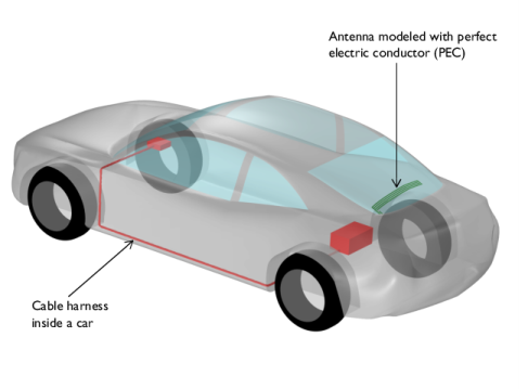
Browse to the model’s Application Libraries folder and double-click the file car_emiemc.mphbin.

Click .

Click the

button in the toolbar.

Sphere 1 (sph1)

In the toolbar, click

In the window for , locate the section.

In the text field, type 4.

Click to expand the section. In the table, enter the following settings:


Layer name	Thickness (m)
Layer 1	0.5

Block 1 (blk1)

In the toolbar, click

In the window for , locate the section.

In the text field, type 8.

In the text field, type 4.

Locate the section. From the list, choose .

In the text field, type -2.

Difference 1 (dif1)

In the toolbar, click

and choose .

Select the object only.

In the window for , locate the section.

Find the subsection. Select the

toggle button.

Select the object only.

Click

Ignore Vertices 1 (igv1)

In the toolbar, click

and choose .

In the window for , locate the section.

Click

In the dialog box, type 110 111 117 118 190 191 in the text field.

Click .

This removes some vertices generating unnecessary finer mesh elements.

In the toolbar, click

Definitions

Create a set of selections before setting up the physics.

Windshield

In the toolbar, click

In the window for , type Windshield in the text field.

Locate the section. From the list, choose .

Click

In the dialog box, type 66-67, 104-107, 127-128, 169-170, 191-196, 202 in the text field.

Click .

Tire

In the toolbar, click

In the window for , type Tire in the text field.

Select Domains 5, 6, 18, and 19 only.

Harness

In the toolbar, click

In the window for , type Harness in the text field.

Select Domains 7–12 and 15–17 only.

Locate the section. From the list, choose .

Perfectly Matched Layer 1 (pml1)

In the toolbar, click

Select Domains 1, 2, 13, and 14 only.

In the window for , locate the section.

From the list, choose .

Electromagnetic Waves, Frequency Domain (emw)

Perfect Electric Conductor 2

In the window, under right-click and choose .

In the window for , locate the section.

Click

In the dialog box, type 9-31, 45-46, 54-60, 88-89, 95-96, 98-103, 108-111, 121-126, 145-155, 172-173, 177-178, 181-182, 185-188, 198-200, 203-206, 208-219 in the text field.

Click .

Perfect Electric Conductor 3

In the toolbar, click

and choose .

In the window for , locate the section.

Click

In the dialog box, type 44, 47, 171, 174 in the text field.

Click .

Perfect Electric Conductor 4

In the toolbar, click

and choose .

In the window for , locate the section.

Click

In the dialog box, type 189-190, 197, 207 in the text field.

Click .

Perfect Electric Conductor 5

In the toolbar, click

and choose .

In the window for , locate the section.

From the list, choose .

Click

In the dialog box, type 79, 142 in the text field.

Click .

Transition Boundary Condition 1

In the toolbar, click

and choose .

In the window for , locate the section.

From the list, choose .

Wave Equation, Electric 2

In the toolbar, click

and choose .

In the window for , locate the section.

From the list, choose .

Locate the section. From the list, choose .

Lumped Port 1

In the toolbar, click

and choose .

Select Boundary 201 only.

For the first port, wave excitation is by default.

Far-Field Domain 1

In the toolbar, click

and choose .

Far-Field Calculation 1

In the window, expand the node, then click .

In the window for , locate the section.

Select the check box.

From the list, choose .

Materials

Material 1 (mat1)

In the window, under right-click and choose .

In the window for , locate the section.

In the table, enter the following settings:


Property	Variable	Value	Unit	Property group
Relative permittivity	epsilonr_iso ; epsilonrii = epsilonr_iso, epsilonrij = 0	1	1	Basic
Relative permeability	mur_iso ; murii = mur_iso, murij = 0	1	1	Basic
Electrical conductivity	sigma_iso ; sigmaii = sigma_iso, sigmaij = 0	0	S/m	Basic

Material 2 (mat2)

Right-click and choose .

In the window for , locate the section.

From the list, choose .

Locate the section. In the table, enter the following settings:


Property	Variable	Value	Unit	Property group
Relative permittivity (real part)	epsilonPrim_iso ; epsilonPrimii = epsilonPrim_iso, epsilonPrimij = 0	2	1	Loss tangent, loss angle
Loss tangent, loss angle	delta	0.00005	rad	Loss tangent, loss angle
Relative permeability	mur_iso ; murii = mur_iso, murij = 0	1	1	Basic

Material 3 (mat3)

Right-click and choose .

In the window for , locate the section.

From the list, choose .

Locate the section. In the table, enter the following settings:


Property	Variable	Value	Unit	Property group
Relative permittivity	epsilonr_iso ; epsilonrii = epsilonr_iso, epsilonrij = 0	4	1	Basic
Relative permeability	mur_iso ; murii = mur_iso, murij = 0	1	1	Basic
Electrical conductivity	sigma_iso ; sigmaii = sigma_iso, sigmaij = 0	0	S/m	Basic