2D Non-Newtonian Slot Die Coating

Achieving uniform coating quality is important in several different industries: from optical coatings, semiconductor and electronics industry, through technologies utilizing thin membranes, to surface treatment of metals. Bad coating quality will compromise the performance of the products, or lead to complete failure in some cases.

Several different coating processes exist. This tutorial investigates the performance of a slot-die coating process, a so-called pre-metered coating method. In this process, the coating fluid is suspended from a thin slot die to a moving substrate. The final coating layer thickness is evaluated from the continuity relationship for a coating liquid. Therefore, the thickness of the liquid layer is determined by the slot gap, the coating fluid inlet velocity and the substrate speed.

The final goal of coating processes is to achieve a defect-free film of a desired thickness. However, manufacturing the uniform coating is not a trivial task, various flow instabilities or defects such as bubbles, ribbing, and rivulets are frequently observed in the process. The die geometry, the size of the slot and height above the substrate, together with the non-Newtonian fluid nature of the coating fluid are important to consider.

This tutorial demonstrates how to model the fluid flow in a polymer slot die coating process using the interface and an inelastic non-Newtonian power law model for the polymer fluid.

Model Definition

Model Geometry

A typical setup of the slot-die coating process is shown in Figure 1.

Figure 1: Typical geometry for a slot-die coating process with the slot die positioned over a substrate.

This model uses a 2D cross section of the die shown in Figure 1, assuming out-of-plane invariance. The inlet for the coating fluid is at the top of the die, as shown in Figure 2, and there are open boundaries at both ends. The bottom boundary is the coating substrate which is moving at the coating velocity.

Figure 2: Model geometry. 2D cross section of a slot die.

The geometrical and material parameters in this model are taken from the Ref. 1.

Domain Equations and Boundary Conditions

The flow in this model is laminar, so a interface will be used together with a interface to track the interface between the air and the polymer fluid. The coupling of these two interfaces is handled by the multiphysics interface. In this interface, you can select which constitutive relationship to use for each of the fluid phases. The air is specified as a Newtonian fluid, and the coating fluid is a non-Newtonian power law fluid.

The inlet fluid velocity is increases smoothly from 0 m/s to 0.1 m/s. Both the upstream and downstream boundaries of the model are specified as open boundaries. The corresponding inlet and outlet boundary conditions must also be set in the interface together with the initial values for both fluids to correctly define the position of the initial interface. For the moving substrate, a moving wall boundary condition with a Navier-Slip condition is used.

Results and Discussion

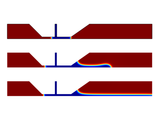
The Figure 3 shows the evolution of the coating fluid interface for t = 0.03 s, t = 0.1 s, and t = 0.2 s.

Figure 3: Coating fluid interface at t = 0.03 s, t = 0.1 s and t = 0.2 s (top to bottom).

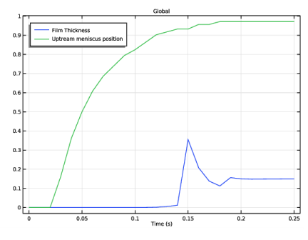
The coating film attains a constant thickness downstream of the die at t = 0.2 s. The film forms upstream and downstream meniscii with the upstream and downstream walls of the die. As the substrate speed increases or the inlet velocity decreases, the upstream meniscus is pulled closer to the slot, eventually causing defects in the coating film. The evolution of the film thickness and position of the upstream meniscus as a function of time is shown in Figure 4.

Figure 4: Film thickness and upstream meniscus position as a function of time.

By changing the geometry, the inlet velocity and wall velocity, it is easy to explore the sensitivity of the design parameters towards the film thickness and coating velocity for a variety of fluid properties in a fast and efficient manner.

Notes About the COMSOL Implementation

The default method for averaging the fluid properties across the interface between the two phases is linear with respect to the volume fraction. When working with fluids that have a large difference in viscosities, switching to a different averaging method increases the performance. In this example, the Heaviside averaging method is applied. The averaged viscosity is defined as

where V2 is the volume fraction of fluid 2, μ1 and μ2 are the viscosities for phase 1 and 2, respectively, and H is a smoothed Heaviside function. The default value for lμ is 0.8. A lower value will sharpen the interface, but also increase the computation time.

In addition, this example demonstrates how to use an add-in to fit measured rheology data to a selected inelastic non-Newtonian fluid model. The add-in utilizes functionality from the Optimization Module. In case you do not have access to this module, you can skip the corresponding part of the instructions.

Reference

1. K.L. Bhamidipati, Detection and elimination of defects during manufacture of high-temperature polymer electrolyte membranes, PhD Thesis, Georgia Institute of Technology, 2011.

Polymer_Flow_Module/Tutorials/slot_die_coating_2d

Modeling Instructions

From the menu, choose .

New

In the window, click

Model Wizard

In the window, click

In the tree, select .

Click .

Click

In the tree, select .

Click

Load the model parameters from a text file.

Global Definitions

Parameters 1

In the window, under click .

In the window for , locate the section.

Click

Browse to the model’s Application Libraries folder and double-click the file slot_die_coating_2d_parameters.txt.

Create a step function to use for ramping up the inlet velocity. To improve convergence, define a smoothing transition zone to gently increase the inlet velocity from zero.

Step 1 (step1)

In the toolbar, click

and choose .

In the window for , type step1 in the text field.

Locate the section. In the text field, type 0.01.

Click to expand the section. In the text field, type 0.02.

Create the geometry by using a rectangle and a polygon.

Geometry 1

In the window, under click .

In the window for , locate the section.

From the list, choose .

Rectangle 1 (r1)

In the toolbar, click

In the window for , locate the section.

In the text field, type W.

In the text field, type Hc.

Locate the section. In the text field, type -W/2.

In the text field, type H.

Add an additional layer at the bottom of the channel. You will use it later to define the initial domain for the coating fluid.

Click to expand the section. In the table, enter the following settings:


Layer name	Thickness (mm)
Layer 1	0.1[mm]

Click

Polygon 1 (pol1)

In the toolbar, click

In the window for , locate the section.

In the table, enter the following settings:


x (mm)	y (mm)
-W/2	H
-W/2-W_ud	H
-W/2-W_ud-tan(alpha_u)*Hc	Hc+H
-W/2-L_u	Hc+H
-W/2-L_u	0
W/2+L_d	0
W/2+L_d	Hc+H
W/2+W_dd+tan(alpha_d)*Hc	Hc+H
W/2+W_dd	H

Click

Click the

button in the toolbar.

Compare the resulting geometry to Figure 2.

Definitions

Next define integration operators. First define an integration coupling that integrates along the outlet boundary, to calculate the film thickness. Then define a coupling operator that integrates along the upstream die lip. You will use it later for the integration of the volume fraction along the boundary to evaluate the location of the upstream meniscus.

Integration 1 (intop1)

In the window, expand the node.

Right-click and choose .

In the window for , locate the section.

From the list, choose .

Select Boundary 16 only.

Integration 2 (intop2)

In the toolbar, click

and choose .

In the window for , locate the section.

From the list, choose .

Select Boundary 5 only.

Add Material

Define the materials for the model — air and a coating fluid.

In the toolbar, click

to open the window.

Go to the window.

In the tree, select .

Click in the window toolbar.

In the toolbar, click

to close the window.

Materials

Coating Fluid

In the window, under right-click and choose .

In the window for , type Coating Fluid in the text field.

The physics interface and the chosen fluid model will suggest which material properties should be defined.

Multiphysics

Two-Phase Flow, Phase Field 1 (tpf1)

In the window, under click .

In the window for , locate the section.

From the list, choose .

Locate the section. From the list, choose .

Find the subsection. From the list, choose .

Locate the section. From the list, choose . In the σ text field, type 0.49.

If you have the Optimiziation module in your license, you may use an add-in to calculate the parameters for the power law fluid model based on measurement data in this example. The instructions in the following section show you how to do this. If you do not have access to that license, you may just use the parameters m=7.77 and n=0.86 for the power law coefficients.

In the toolbar, click

and choose .

Add-in Libraries

In the window, click

In the tree, select .

In the tree, select the check box for the node .

Click

Root

In the toolbar, click

and choose .

Global Definitions

Inelastic Non-Newtonian Fluid Parameter Estimation 1

In the window, under click .

In the window for , click

Browse to the model’s Application Libraries folder and double-click the file slot_die_coating_2d_viscosity_input.txt.

Click to start the parameter estimation.

The power law parameters can now be found in the global parameters table, and thus be used in the material node for the Coating Fluid.

Materials

Coating Fluid (mat2)

In the window, under click .

In the window for , locate the section.

In the table, enter the following settings:


Property	Variable	Value	Unit	Property group
Density	rho	1400	kg/m³	Basic
Fluid consistency coefficient	m_pow	m_powerLaw	Pa·s	Power law
Flow behavior index	n_pow	n_powerLaw	1	Power law

To avoid having the optimization component in the model, use the button in the add-in to clean up the model tree.

Now, set up the physics of the problem by defining the domain physics conditions and the boundary conditions.

Laminar Flow (spf)

Wall 2

In the window, under right-click and choose .

Select Boundary 2 only.

In the window for , locate the section.

From the list, choose .

Click to expand the section. Select the check box.

In the Uw text field, type -U_wall.

Inlet 1

In the toolbar, click

and choose .

Select Boundary 10 only.

In the window for , locate the section.

In the U0 text field, type step1(t[1/s])*U_in.

Open Boundary 1

In the toolbar, click

and choose .

Select Boundaries 1 and 16 only.

The initial interface between the coating fluid and air is automatically assigned to the boundaries between the two initial value domains. Set up the initial coating fluid domain in the inlet channel.

Phase Field (pf)

Initial Values, Fluid 2

In the window, under click .

Select Domain 3 only.

Wetted Wall 1

In the window, click .

In the window for , locate the section.

In the θw text field, type 68.5[deg].

Inlet 1

In the toolbar, click

and choose .

In the window for , locate the section.

From the list, choose ϕ .

Select Boundary 10 only.

Outlet 1

In the toolbar, click

and choose .

Select Boundaries 1 and 16 only.

Wetted Wall 2

In the toolbar, click

and choose .

Select Boundary 2 only.

In the window for , locate the section.

In the θw text field, type 74[deg].

When working with fluids that have large viscosity and density ratios, switching from the default linear method for the properties averaging can increase the performance.

Multiphysics

Two-Phase Flow, Phase Field 1 (tpf1)

Click the

button in the toolbar.

In the dialog box, in the tree, select the check box for the node .

Click .

In the window, under click .

In the window for , click to expand the section.

From the list, choose .

In the lρ text field, type 0.9.

From the list, choose .

In the lμ text field, type 0.9.

The mixing parameter can be decreased to sharpen the interface, but that will increase the computation time for this example.

If you want to inspect the progress of the fluids during the simulation, you can enable the plot while solving option in the node. By calculating the initial values first, the solver sequence and default plots will be generated. In the following section you generate the default plot groups and use one of them for plotting the volume fraction while solving. Note that plot while solving in general will affect the computation time slightly since the plot needs to be updated in each timestep.

Study 1

In the toolbar, click