PDF

Rubber Injection Molding
Introduction
Injection molding is a popular way of producing devices and equipment. A polymer fluid is injected into a mold, where it eventually will set to form the desired shape.
This tutorial demonstrates how to model the fluid flow in a rubber injection molding process of an automotive vibration damper using the Laminar Two-Phase Flow, Phase Field interface and an inelastic non-Newtonian power law model for the rubber. The model geometry and material parameters are inspired from Ref. 1.
Model Definition
Model geometry
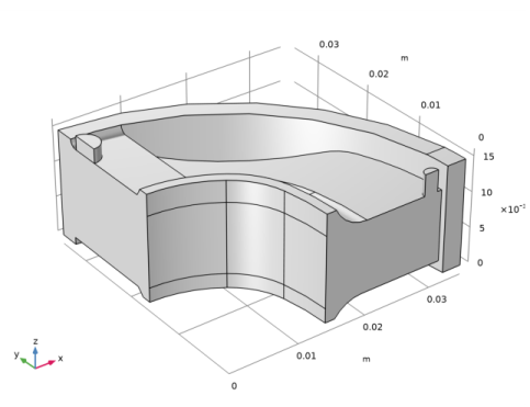
The geometry of the vibration damper is an imported CAD file where only the fluid domains are present. A quarter symmetry is used to reduce the computation time. The geometry can be seen in Figure 1.
Figure 1: Model geometry. A quarter piece of the fluid volume of an automotive vibration damper. The fluid inlet can be seen at the top of the small cylinder to the left. While the outlets are to the right in the figure.
Domain equations and boundary conditions
The flow in this model is laminar, so a Laminar Flow interface will be used together with a Phase Field interface for the tracking of the interface between the air and the rubber fluid. The coupling of these two interfaces is handled by the Two-Phase Flow, Phase Field multiphysics interface. In this multiphysics interface, you can also select which constitutive relationship to use for each of the fluid phases. The air is specified as a Newtonian fluid, and the rubber is a non-Newtonian power law fluid.
A small portion of the inlet channel is set up to contain rubber initially. This will automatically define the initial interface between rubber and air.
At the rubber inlet, the fluid velocity is increased smoothly from 0 at = 0, and the outlets have a uniform pressure, = 0. The corresponding inlet and outlet boundary conditions must also be set in the Phase Field interface together with the initial values for both fluids, so that the initial interface is correctly defined.
The symmetry planes are defined as Symmetry in both the Laminar flow interface and the Phase field interface. All other boundaries are solid walls described by a no-slip boundary condition.
Results and Discussion
Figure 2-Figure 5 show the propagation of the rubber front as time progresses from t = 1s, t = 4s, t = 8s and t = 16s.
Figure 2: Rubber front after t = 1s.
Figure 3: Rubber front after t = 4s
.
Figure 4: Rubber front after t = 8s.
Figure 5: Rubber front after t = 16s.
The mold is almost completely filled after 16s. The small remaining void near the bottom corner might indicate that the mold design needs to be modified.
Notes About the COMSOL Implementation
The default method for averaging the fluid properties across the interface between the two phases is linear with respect to the volume fraction. When working with fluids that have a large difference in viscosities, switching to a different averaging method increases the performance. This example utilizes the Heaviside averaging method.
Reference
1. M. Erfanian, M. Anbarsooz, and M. Moghima, “A three dimensional simulation of a rubber curing process considering variable order of reaction,” Applied Mathematical Modeling, vol. 40, pp. 8592–8604, 2016.
Application Library path: Polymer_Flow_Module/Tutorials/rubber_injection_molding
Modeling Instructions
From the File menu, choose New.
New
In the New window, click  Model Wizard.
Model Wizard
1
In the Model Wizard window, click  3D.
2
In the Select Physics tree, select Fluid Flow>Multiphase Flow>Two-Phase Flow, Phase Field>Laminar Flow.
3
Click Add.
4
Click  Study.
5
In the Select Study tree, select Preset Studies for Selected Multiphysics>Time Dependent with Phase Initialization.
6
Global Definitions
Parameters 1
1
In the Model Builder window, under Global Definitions click Parameters 1.
2
In the Settings window for Parameters, locate the Parameters section.
3
Geometry 1
Import 1 (imp1)
1
In the Home toolbar, click  Import.
2
In the Settings window for Import, locate the Import section.
3
Click Browse.
4
5
Click Import.
Form Union (fin)
1
In the Model Builder window, click Form Union (fin).
2
In the Settings window for Form Union/Assembly, click  Build Selected.
Materials
Air
1
In the Model Builder window, under Component 1 (comp1) right-click Materials and choose Blank Material.
2
In the Settings window for Material, type Air in the Label text field.
3
Locate the Material Contents section. In the table, enter the following settings:
It is convenient to add an empty material and assign the material to the phase in the Two-Phase Flow, Phase Field (tpf1) interface defined as an inelastic non-Newtonian fluid. This will automatically enable the right fields for the corresponding fluid properties in the material node.
Rubber
1
Right-click Materials and choose Blank Material.
2
In the Settings window for Material, type Rubber in the Label text field.
Multiphysics
Two-Phase Flow, Phase Field 1 (tpf1)
1
Click the  Show More Options button in the Model Builder toolbar.
2
In the Show More Options dialog box, in the tree, select the check box for the node Physics>Advanced Physics Options.
3
4
In the Model Builder window, under Component 1 (comp1)>Multiphysics click Two-Phase Flow, Phase Field 1 (tpf1).
5
In the Settings window for Two-Phase Flow, Phase Field, locate the Fluid 1 Properties section.
6
From the Fluid 1 list, choose Air (mat1).
7
Locate the Fluid 2 Properties section. From the Fluid 2 list, choose Rubber (mat2).
8
Find the Constitutive relation subsection. From the list, choose Inelastic non-Newtonian.
9
Locate the Surface Tension section. Clear the Include surface tension force in momentum equation check box.
10
Click to expand the Advanced Settings section. From the Density averaging list, choose Heaviside function.
11
From the Viscosity averaging list, choose Heaviside function.
The default method for averaging the viscosity across the interface between the two phases is linear with respect to the volume fraction. When working with fluids that have a large difference in viscosities, switching to a different averaging method increases the performance. In this model we use the Heaviside averaging method. The mixing parameter can be made smaller to sharpen the interface, but that will increase the computation time.
Materials
Rubber (mat2)
1
In the Model Builder window, under Component 1 (comp1)>Materials click Rubber (mat2).
2
In the Settings window for Material, locate the Material Contents section.
3
At the start-up of a transient simulation of a filling process you can assume that the initial velocity in the domain is zero. To get consistent initial values, the initial velocity at the inlet should also be zero. Use a step function as described in the section below to ramp up the inlet velocity.
Definitions
Step 1 (step1)
1
In the Model Builder window, expand the Component 1 (comp1)>Definitions node.
2
Right-click Definitions and choose Functions>Step.
3
In the Settings window for Step, locate the Parameters section.
4
In the Location text field, type 0.05.
5
Click to expand the Smoothing section. In the Size of transition zone text field, type 0.095.
Variables 1
1
Right-click Definitions and choose Variables.
2
In the Settings window for Variables, locate the Variables section.
3
Laminar Flow (spf)
Inlet 1
1
In the Model Builder window, under Component 1 (comp1) right-click Laminar Flow (spf) and choose Inlet.
2
3
In the Settings window for Inlet, locate the Velocity section.
4
In the U0 text field, type U_in.
Outlet 1
1
In the Physics toolbar, click  Boundaries and choose Outlet.
2
Symmetry 1
1
In the Physics toolbar, click  Boundaries and choose Symmetry.
2
The initial interface between the rubber fluid and air is automatically assigned to the boundaries between the two initial value domains. Assign the initial values of fluid two to the small domain close to the inlet.
Phase Field (pf)
Initial Values, Fluid 2
1
In the Model Builder window, under Component 1 (comp1)>Phase Field (pf) click Initial Values, Fluid 2.
2
Inlet 1
1
In the Physics toolbar, click  Boundaries and choose Inlet.
2
3
In the Settings window for Inlet, locate the Phase Field Condition section.
4
From the list, choose Fluid 2 (ϕ = 1).
Outlet 1
1
In the Physics toolbar, click  Boundaries and choose Outlet.
2
Symmetry 1
1
In the Physics toolbar, click  Boundaries and choose Symmetry.
2
When working with two-phase flows, the mesh should be fine enough to resolve the initial fluid interface. It is also advantageous to have a relatively uniform mesh element size in the domain. Modify the default mesh sequence to achieve a better mesh for this model.
Mesh 1
1
In the Model Builder window, under Component 1 (comp1) click Mesh 1.
2
In the Settings window for Mesh, locate the Mesh Settings section.
3
From the Sequence type list, choose User-controlled mesh.
Size
1
In the Model Builder window, under Component 1 (comp1)>Mesh 1 click Size.
2
In the Settings window for Size, locate the Element Size section.
3
Click the Custom button.
4
Locate the Element Size Parameters section. In the Maximum element size text field, type 0.00125/2.
Size 1
1
In the Model Builder window, click Size 1.
2
In the Settings window for Size, locate the Element Size section.
3
Click the Custom button.
4
Locate the Element Size Parameters section. Select the Maximum element size check box.
5
6
Click  Build All.
Study 1
Step 2: Time Dependent
1
In the Model Builder window, under Study 1 click Step 2: Time Dependent.
2
In the Settings window for Time Dependent, locate the Study Settings section.
3
In the Output times text field, type range(0,1,16).
4
In the Home toolbar, click  Compute.
Results
Injected fluid
1
In the Home toolbar, click  Add Plot Group and choose 3D Plot Group.
2
In the Settings window for 3D Plot Group, locate the Data section.
3
From the Time (s) list, choose 8.
4
In the Label text field, type Injected fluid.
Volume 1
1
Right-click Injected fluid and choose Volume.
2
In the Settings window for Volume, locate the Expression section.
3
In the Expression text field, type 1.
4
Locate the Coloring and Style section. From the Coloring list, choose Uniform.
5
From the Color list, choose Cyan.
6
Click to expand the Title section. From the Title type list, choose Manual.
7
In the Title text area, type Rubber fluid in mold.
Filter 1
1
Right-click Volume 1 and choose Filter.
2
In the Settings window for Filter, locate the Element Selection section.
3
In the Logical expression for inclusion text field, type pf.Vf2>0.5.
Injected fluid
1
In the Model Builder window, click Injected fluid.
2
In the Settings window for 3D Plot Group, click to expand the Title section.
Surface 1
1
Right-click Injected fluid and choose Surface.
2
In the Settings window for Surface, locate the Expression section.
3
In the Expression text field, type 1.
4
Locate the Coloring and Style section. From the Coloring list, choose Uniform.
5
From the Color list, choose Gray.
6
Click to expand the Title section. From the Title type list, choose None.
Transparency 1
1
Right-click Surface 1 and choose Transparency.
2
In the Settings window for Transparency, locate the Transparency section.
3
Set the Transparency value to 0.75.
Injected fluid
1
In the Model Builder window, click Injected fluid.
2
In the Injected fluid toolbar, click  Plot.