PDF

In-Plane Microwave Plasma
Introduction
Wave-heated discharges can be very simple, such as when a plane wave is guided into a reactor using a waveguide, or very complicated, such as in the case with ECR (electron cyclotron resonance) reactors. In this simple example, a wave is launched down a waveguide where it intersects a flowing gas at low pressure, resulting in formation of an argon plasma. Microwave plasmas typically have high number density without requiring significant power absorption. The plasma potential is also quite low compared to capacitive or DC discharges. Therefore, microwave plasmas share many of the characteristics of inductive discharges.
Figure 1: Diagram of geometry modeled. A TE or TM mode wave enters from the top port and intersects the gas flow leading to the formation of a plasma.
Note: The model requires the Plasma Module and RF Module.
Model Definition
The electron density and mean electron energy are computed by solving a pair of drift-diffusion equations for the electron density and mean electron energy. Convection of electrons due to fluid motion is neglected. For detailed information on electron transport, see Theory for the Drift Diffusion Interface in the Plasma Module User’s Guide.
The electron source Re and the energy loss due to inelastic collisions Rε are defined later. The electron diffusivity, energy mobility, and energy diffusivity are computed from the electron mobility using:
The source coefficients in the above equations are determined by the plasma chemistry using rate coefficients. Suppose that there are M reactions that contribute to the growth or decay of electron density and P inelastic electron-neutral collisions. In general, P >> M. In the case of rate coefficients, the electron source term is given by:
where xj is the mole fraction of the target species for reaction j, kj is the rate coefficient for reaction j (SI unit: m3/s), and Nn is the total neutral number density (SI unit: 1/m3). The electron energy loss is obtained by summing the collisional energy loss over all reactions:
where Δεj is the energy loss from reaction j (SI unit: V). The rate coefficients can be computed from cross section data by the following integral:
where γ = (2q/me)1/2 (SI unit: C1/2/kg1/2), me is the electron mass (SI unit: kg), ε is energy (SI unit: V), σk is the collision cross section (SI unit: m2), and f is the electron energy distribution function. In this case, a Maxwellian EEDF is assumed.
For nonelectron species, the following equation is solved for the mass fraction of each species. For detailed information on the transport of the nonelectron species, see Theory for the Heavy Species Transport Interface in the Plasma Module User’s Guide.
The electrostatic field is computed using the following equation:
The space charge density ρ is automatically computed based on the plasma chemistry specified in the model using the formula:
For detailed information about electrostatics see Theory for the Electrostatics Interface in the Plasma Module User’s Guide.
In a microwave reactor the high frequency electric field is computed in the frequency domain using the following equation:
The relationship between the plasma current density and the electric field becomes more complicated in the presence of a DC magnetic field. The following equation defines this relationship:
Here, σ is the plasma conductivity tensor, which is a function of the electron density, collision frequency, and magnetic flux density. Using the definitions:
where q is the electron charge, me is the electron mass, ne is the collision frequency, and ω is the angular frequency of the electromagnetic field. In this example, the inverse of the plasma conductivity is diagonal because there is no external DC magnetic field:
The gas flow is modeled assuming a constant velocity in the x-direction.
plasma chemistry
The chemical mechanism for the plasma consists of only 3 species and 7 reactions (electron impact cross-section are obtained from Ref. 2):
Stepwise ionization (reaction 5) can play an important role in sustaining low pressure argon discharges. Excited argon atoms are consumed via superelastic collisions with electrons, quenching with neutral argon atoms, ionization or Penning ionization where two metastable argon atoms react to form a neutral argon atom, an argon ion and an electron. Reaction number 7 is responsible for heating of the gas. The 11.5 eV of energy which was consumed in creating the electronically excited argon atom is returns to the gas as thermal energy when the excited metastable quenches. In addition to volumetric reactions, the following surface reactions are implemented:
When a metastable argon atom makes contact with the wall, it reverts to the ground state argon atom with some probability (the sticking coefficient).
electrical excitation
The plasma is sustained through absorption of electromagnetic waves. The Port boundary condition is used to excite the plasma. A total absorbed power of 30 W is fed into the port.
In a second study, the electrical excitation is changed to the TM mode, where the electric field has only an in-plane component. The total absorbed power is the same as the TE mode case.
Results and Discussion
The electron density is plotted in Figure 2 and peaks slightly downstream of the crossing point. The electron density is also slightly asymmetric in the y-plane due to the fact that the electromagnetic waves are absorbed asymmetrically. The electron “temperature” is plotted in Figure 3. The electron temperature is relatively low everywhere, in part due to the high operating pressure (1 Torr). The electron “temperature” peaks directly underneath the waveguide where the wave is absorbed. The norm of the electric field can be seen in Figure 5. The electric field is high inside the waveguide and there are no losses. Once the wave is exposed to the plasma, the energy is absorbed by the electrons, raising the electron temperature enough to generate new electrons through ionization. The ionization rate is high enough to sustain the plasma. The contour of the critical plasma density is also plotted in Figure 5. The electromagnetic wave cannot penetrate into regions exceeding the critical plasma density. Since the electron “temperature” is relatively low, one would expect the plasma potential to be low. The plasma potential is plotted in Figure 4 and is only around 10 volts.
In the TE mode, electrons do not experience any change in the high-frequency electric field during the microwave time scale. This means that the phase coherence between the electrons and electromagnetic waves is only destroyed through collisions with the background gas. The loss of phase coherence between the electrons and high-frequency fields is what results in energy gain for the electrons. Therefore, the momentum collision frequency is simply given by:
where νe is the collision frequency between the electrons and neutrals.
When switching to the TM mode, the electron density, electron “temperature” and plasma potential are quite similar to the TE mode case. This can be seen in Figure 7, Figure 8 and Figure 9. The electric field is very different however, Figure 9. The electric field cannot penetrate past the contour of critical electron density, and has its greatest magnitude in this location. The power deposition, Figure 10 is also highly localized to the contour of critical electron density. The TM mode causes in-plane motion of the electrons on the microwave time scale, so in regions where the high-frequency electric field is significant (the contour where the electron density is equal to the critical density), the time-averaged electric field experienced by the electrons may be nonzero. This destroys the phase coherence between the electrons and the fields, causing the electrons to gain energy. This is an example of a nonlocal kinetic effect, which is difficult to approximate with a fluid model. However, since this effect is similar to collisions with a background gas, the nonlocal effects can be approximated by adding an effective collision frequency to the momentum collision frequency:
where νeff is the effective collision frequency to account for nonlocal effects. In this example, since the Doppler broadening parameter is set to 20, this corresponds to an effective collision frequency of:
Figure 2: Plot of the electron density.
Figure 3: Plot of the electron temperature in the reactor.
Figure 4: Plot of the plasma potential in the reactor.\
Figure 5: Plot of the electric field norm. The white contour represents the critical plasma density, where the electron density is equal to 7.6E16[1/m3].
Figure 6: Plot of the power deposition into the plasma. The white contour represents the critical plasma density, where the electron density is equal to 7.6E16 1/m3.
Figure 7: Electron density for the TM mode case.
Figure 8: Plot of the electron temperature for the TM mode case.
Figure 9: Close up of the high frequency electric field norm for the TM mode case.
Figure 10: Close up of the power deposition into the plasma for the TM mode case.
Reference
1. M.A. Lieberman and A.J. Lichtenberg, Principles of Plasma Discharges and Materials Processing, John Wiley & Sons, 2005.
2. Phelps database, www.lxcat.net, retrieved 2017.
Application Library path: Plasma_Module/Wave-Heated_Discharges/inplane_microwave_plasma
Modeling Instructions
From the File menu, choose New.
New
In the New window, click  Model Wizard.
Model Wizard
1
In the Model Wizard window, click  2D.
2
In the Select Physics tree, select Plasma>Microwave Plasma.
3
Click Add.
4
Click  Study.
5
In the Select Study tree, select Preset Studies for Selected Multiphysics>Frequency-Transient.
6
Global Definitions
Parameters 1
1
In the Model Builder window, under Global Definitions click Parameters 1.
2
In the Settings window for Parameters, locate the Parameters section.
3
Geometry 1
Rectangle 1 (r1)
1
In the Geometry toolbar, click  Rectangle.
2
In the Settings window for Rectangle, locate the Size and Shape section.
3
In the Width text field, type 0.05.
4
In the Height text field, type 0.1.
5
Click  Build All Objects.
Rectangle 2 (r2)
1
In the Geometry toolbar, click  Rectangle.
2
In the Settings window for Rectangle, locate the Size and Shape section.
3
In the Width text field, type 0.25.
4
In the Height text field, type 0.05.
5
Locate the Position section. In the x text field, type -0.1.
6
In the y text field, type 0.1.
Rectangle 3 (r3)
1
In the Geometry toolbar, click  Rectangle.
2
In the Settings window for Rectangle, locate the Size and Shape section.
3
In the Width text field, type 0.05.
4
In the Height text field, type 0.1.
5
Locate the Position section. In the y text field, type 0.15.
6
Click  Build All Objects.
7
Click the  Zoom Extents button in the Graphics toolbar.
Definitions
Walls
1
In the Definitions toolbar, click  Explicit.
2
In the Settings window for Explicit, locate the Input Entities section.
3
From the Geometric entity level list, choose Boundary.
4
5
Right-click Explicit 1 and choose Rename.
6
In the Rename Explicit dialog box, type Walls in the New label text field.
7
Plasma (plas)
1
In the Settings window for Plasma, locate the Domain Selection section.
2
Click  Clear Selection.
3
Cross Section Import 1
1
Right-click Component 1 (comp1)>Plasma (plas) and choose Global>Cross Section Import.
2
In the Settings window for Cross Section Import, locate the Cross Section Import section.
3
Click Browse.
4
5
Click Import.
Reaction 1
1
In the Physics toolbar, click  Domains and choose Reaction.
2
In the Settings window for Reaction, locate the Reaction Formula section.
3
In the Formula text field, type Ars+Ars=>e+Ar+Ar+.
4
Locate the Reaction Parameters section. In the kf text field, type 3.734E8.
Reaction 2
1
In the Physics toolbar, click  Domains and choose Reaction.
2
In the Settings window for Reaction, locate the Reaction Formula section.
3
In the Formula text field, type Ars+Ar=>Ar+Ar.
4
Locate the Reaction Parameters section. In the kf text field, type 1807.
Species: Ar
1
In the Model Builder window, click Species: Ar.
2
In the Settings window for Species, locate the Species Formula section.
3
Select the From mass constraint check box.
Species: Ar+
1
In the Model Builder window, click Species: Ar+.
2
In the Settings window for Species, locate the Species Formula section.
3
Select the Initial value from electroneutrality constraint check box.
Surface Reaction 1
1
In the Physics toolbar, click  Boundaries and choose Surface Reaction.
2
In the Settings window for Surface Reaction, locate the Reaction Formula section.
3
In the Formula text field, type Ars=>Ar.
4
Locate the Boundary Selection section. From the Selection list, choose Walls.
Surface Reaction 2
1
In the Physics toolbar, click  Boundaries and choose Surface Reaction.
2
In the Settings window for Surface Reaction, locate the Reaction Formula section.
3
In the Formula text field, type Ar+=>Ar.
4
Locate the Boundary Selection section. From the Selection list, choose Walls.
5
In the Model Builder window, click Plasma (plas).
6
In the Settings window for Plasma, locate the Transport Settings section.
7
Find the Include subsection. Select the Convection check box.
8
Locate the Plasma Properties section. Select the Use reduced electron transport properties check box.
Plasma Model 1
1
In the Model Builder window, click Plasma Model 1.
2
In the Settings window for Plasma Model, locate the Model Inputs section.
3
Specify the u vector as
4
In the T text field, type 350.
5
In the pA text field, type 1[torr].
6
Locate the Electron Density and Energy section. In the μeNn text field, type 4E24.
Initial Values 1
1
In the Model Builder window, click Initial Values 1.
2
In the Settings window for Initial Values, locate the Initial Values section.
3
In the ne,0 text field, type 1E17.
Wall 1
1
In the Physics toolbar, click  Boundaries and choose Wall.
2
In the Settings window for Wall, locate the Boundary Selection section.
3
From the Selection list, choose Walls.
Ground 1
1
In the Physics toolbar, click  Boundaries and choose Ground.
2
In the Settings window for Ground, locate the Boundary Selection section.
3
From the Selection list, choose Walls.
Electron Outlet 1
1
In the Physics toolbar, click  Boundaries and choose Electron Outlet.
2
Species: Ars
In the Model Builder window, click Species: Ars.
Outflow 1
1
In the Physics toolbar, click  Attributes and choose Outflow.
2
In the Settings window for Outflow, locate the Boundary Selection section.
3
Click  Clear Selection.
4
Species: Ar+
In the Model Builder window, click Species: Ar+.
Outflow 1
1
In the Physics toolbar, click  Attributes and choose Outflow.
2
In the Settings window for Outflow, locate the Boundary Selection section.
3
Click  Clear Selection.
4
Electromagnetic Waves, Frequency Domain (emw)
1
In the Model Builder window, under Component 1 (comp1) click Electromagnetic Waves, Frequency Domain (emw).
2
In the Settings window for Electromagnetic Waves, Frequency Domain, locate the Components section.
3
From the Electric field components solved for list, choose Out-of-plane vector.
Port 1
1
In the Physics toolbar, click  Boundaries and choose Port.
2
3
In the Settings window for Port, locate the Port Properties section.
4
From the Type of port list, choose Rectangular.
5
Select the Enable active port feedback check box.
6
In the Pdep text field, type P0.
Materials
Material 1 (mat1)
1
In the Model Builder window, under Component 1 (comp1) right-click Materials and choose Blank Material.
2
3
In the Settings window for Material, locate the Material Contents section.
4
Mesh 1
Boundary Layers 1
1
In the Mesh toolbar, click  Boundary Layers.
2
In the Settings window for Boundary Layers, locate the Domain Selection section.
3
From the Geometric entity level list, choose Domain.
4
Boundary Layer Properties
1
In the Model Builder window, click Boundary Layer Properties.
2
In the Settings window for Boundary Layer Properties, locate the Boundary Selection section.
3
From the Selection list, choose Walls.
Free Triangular 1
In the Mesh toolbar, click  Free Triangular.
Size
1
In the Model Builder window, click Size.
2
In the Settings window for Size, locate the Element Size section.
3
From the Calibrate for list, choose Plasma.
4
From the Predefined list, choose Fine.
5
Click  Build All.
Study 1
Step 1: Frequency-Transient
1
In the Model Builder window, under Study 1 click Step 1: Frequency-Transient.
2
In the Settings window for Frequency-Transient, locate the Study Settings section.
3
In the Output times text field, type 0.
4
Click  Range.
5
In the Range dialog box, choose Number of values from the Entry method list.
6
In the Start text field, type -8.
7
In the Stop text field, type -2.
8
In the Number of values text field, type 31.
9
From the Function to apply to all values list, choose exp10(x) – Exponential function (base 10).
10
Click Add.
11
In the Settings window for Frequency-Transient, locate the Study Settings section.
12
In the Frequency text field, type 2.45[GHz].
13
In the Home toolbar, click  Compute.
Results
Contour 1
1
In the Model Builder window, right-click Electric Field (emw) and choose Contour.
2
In the Settings window for Contour, locate the Levels section.
3
From the Entry method list, choose Levels.
4
In the Levels text field, type 7.6E16.
5
Locate the Coloring and Style section. Clear the Color legend check box.
6
From the Coloring list, choose Uniform.
7
From the Color list, choose White.
8
In the Electric Field (emw) toolbar, click  Plot.
Resistive Heating
1
Right-click Electric Field (emw) and choose Duplicate.
2
Right-click Electric Field (emw) 1 and choose Rename.
3
In the Rename 2D Plot Group dialog box, type Resistive Heating in the New label text field.
4
Surface
1
In the Model Builder window, expand the Resistive Heating node, then click Surface.
2
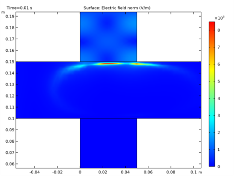
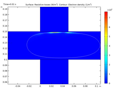
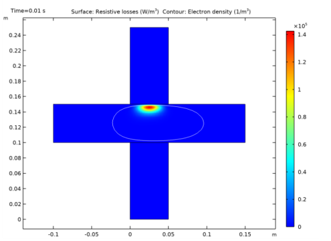
In the Settings window for Surface, click Replace Expression in the upper-right corner of the Expression section. From the menu, choose Component 1 (comp1)>Electromagnetic Waves, Frequency Domain>Heating and losses>emw.Qrh - Resistive losses - W/m³.
3
In the Resistive Heating toolbar, click  Plot.
Now change to the in-plane electric field, which makes the problem much more difficult to solve. This is because all the power will be absorbed on the contour of critical electron density. Setting a Doppler broadening parameter of 20 smooths out the region over which power is deposited to help with convergence.
Multiphysics
Plasma Conductivity Coupling 1 (pcc1)
1
In the Model Builder window, under Component 1 (comp1)>Multiphysics click Plasma Conductivity Coupling 1 (pcc1).
2
In the Settings window for Plasma Conductivity Coupling, locate the Compute Tensor Plasma Conductivity section.
3
Select the Compute tensor plasma conductivity check box.
4
In the δ text field, type 20.
Electromagnetic Waves, Frequency Domain (emw)
1
In the Model Builder window, under Component 1 (comp1) click Electromagnetic Waves, Frequency Domain (emw).
2
In the Settings window for Electromagnetic Waves, Frequency Domain, locate the Components section.
3
From the Electric field components solved for list, choose In-plane vector.
Add Study
1
In the Home toolbar, click  Add Study to open the Add Study window.
2
Go to the Add Study window.
3
Find the Studies subsection. In the Select Study tree, select Preset Studies for Selected Multiphysics>Frequency-Transient.
4
Click Add Study in the window toolbar.
5
In the Home toolbar, click  Add Study to close the Add Study window.
Study 2
Step 1: Frequency-Transient
1
In the Settings window for Frequency-Transient, locate the Study Settings section.
2
In the Output times text field, type 0.
3
Click  Range.
4
In the Range dialog box, choose Number of values from the Entry method list.
5
In the Start text field, type -8.
6
In the Stop text field, type -2.
7
In the Number of values text field, type 31.
8
From the Function to apply to all values list, choose exp10(x) – Exponential function (base 10).
9
Click Add.
10
In the Settings window for Frequency-Transient, locate the Study Settings section.
11
In the Frequency text field, type 2.45[GHz].
12
In the Home toolbar, click  Compute.
Results
Electric Field (emw) 1
1
In the Model Builder window, click Electric Field (emw) 1.
2
In the Electric Field (emw) 1 toolbar, click  Plot.
3
Click the  Zoom In button in the Graphics toolbar.
Resistive Heating 1
1
In the Model Builder window, right-click Resistive Heating and choose Duplicate.
2
In the Settings window for 2D Plot Group, locate the Data section.
3
From the Dataset list, choose Study 2/Solution 2 (sol2).
4
In the Resistive Heating 1 toolbar, click  Plot.
Port Power
1
In the Home toolbar, click  Add Plot Group and choose 1D Plot Group.
2
In the Settings window for 1D Plot Group, type Port Power in the Label text field.
Global 1
1
Right-click Port Power and choose Global.
2
In the Settings window for Global, click Replace Expression in the upper-right corner of the y-Axis Data section. From the menu, choose Component 1 (comp1)>Electromagnetic Waves, Frequency Domain>Global>emw.port1.Pin - Port input power - W/m.
3
In the Port Power toolbar, click  Plot.
4
Click to expand the Legends section. From the Legends list, choose Manual.
5
6
Click the  x-Axis Log Scale button in the Graphics toolbar.
Port Power
1
In the Model Builder window, click Port Power.
2
In the Settings window for 1D Plot Group, locate the Legend section.
3
From the Position list, choose Upper left.
Global 2
1
In the Model Builder window, under Results>Port Power right-click Global 1 and choose Duplicate.
2
In the Settings window for Global, locate the Data section.
3
From the Dataset list, choose Study 2/Solution 2 (sol2).
4
Locate the Legends section. In the table, enter the following settings:
5
Click to expand the Title section. From the Title type list, choose None.
6
In the Port Power toolbar, click  Plot.