|
|
|


|
1
|
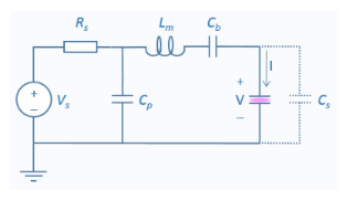
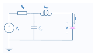
In the Model Wizard window, The model is set up in an identical way to the computing plasma impedance model, except an external circuit is used to drive the discharge.
|
|
2
|
click
|
|
3
|
|
4
|
Click Add.
|
|
5
|
Click
|
|
6
|
|
7
|
Click
|
|
1
|
|
2
|
|
42.696 Ω
|
|||
|
-156.62 Ω
|
|||
|
50 Ω
|
|||
|
174.28 Ω
|
|||
|
1
|
|
2
|
|
4
|
|
5
|
|
1
|
|
2
|
|
3
|
|
4
|
|
5
|
|
6
|
Locate the Plasma Properties section. Select the Use reduced electron transport properties check box.
|
|
1
|
|
2
|
|
3
|
Click Browse.
|
|
1
|
|
2
|
|
3
|
|
4
|
|
1
|
|
2
|
|
3
|
|
1
|
|
2
|
|
3
|
|
4
|
|
5
|
Click to collapse the Species Formula section. Click to expand the Mobility and Diffusivity Expressions section. From the Specification list, choose Specify mobility, compute diffusivity.
|
|
6
|
|
7
|
Click to expand the Mobility Specification section. From the Specify using list, choose Helium ion in helium.
|
|
1
|
|
2
|
|
3
|
|
4
|
|
1
|
|
2
|
|
3
|
|
4
|
|
5
|
|
6
|
|
7
|
|
1
|
|
2
|
|
3
|
|
4
|
|
1
|
|
2
|
|
3
|
|
1
|
|
1
|
|
3
|
|
4
|
|
5
|
|
6
|
|
7
|
|
8
|
|
9
|
|
10
|
|
11
|
|
1
|
|
2
|
|
3
|
|
4
|
|
5
|
|
6
|
|
7
|
|
1
|
|
2
|
|
3
|
|
4
|
|
1
|
|
2
|
|
3
|
|
4
|
Click
|
|
7
|
Click
|
|
8
|
|
9
|
|
10
|
|
11
|
|
12
|
Click Replace.
|
|
13
|
|
15
|
|
1
|
|
2
|
|
1
|
|
2
|
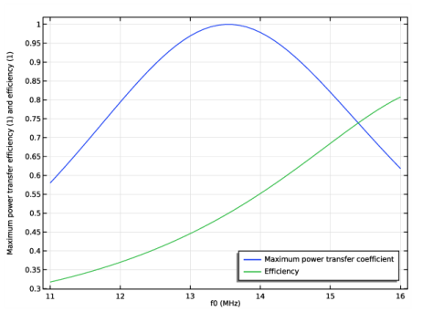
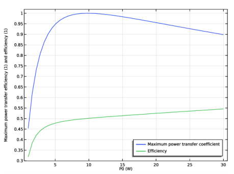
In the Settings window for Global, click Replace Expression in the upper-right corner of the y-Axis Data section. From the menu, choose Component 1 (comp1)>Plasma, Time Periodic>Metal Contact 1>Circuit variables>ptp.mct1.alphaP - Maximum power transfer coefficient.
|
|
3
|
Click Add Expression in the upper-right corner of the y-Axis Data section. From the menu, choose Component 1 (comp1)>Plasma, Time Periodic>Metal Contact 1>Circuit variables>ptp.mct1.etaP - Efficiency.
|
|
4
|
|
1
|
|
2
|
|
3
|
|
4
|
In the associated text field, type Maximum power transfer efficiency (1) and efficiency (1).
|
|
5
|
|
6
|
|
7
|
|
8
|
|
1
|
|
2
|
|
3
|
Find the Studies subsection. In the Select Study tree, select Preset Studies for Selected Physics Interfaces>Time Periodic.
|
|
4
|
|
5
|
|
1
|
|
2
|
|
3
|
Click
|
|
6
|
Click
|
|
7
|
|
8
|
|
9
|
|
10
|
|
11
|
Click Replace.
|
|
12
|
|
14
|
|
15
|
|
16
|
|
17
|
|
18
|
|
19
|
|
1
|
|
2
|
|
3
|
|
1
|
|
2
|
|
1
|
|
2
|
Find the Studies subsection. In the Select Study tree, select Preset Studies for Selected Physics Interfaces>Time Periodic.
|
|
3
|
|
4
|
|
1
|
|
2
|
|
3
|
Click
|
|
6
|
Click
|
|
7
|
|
8
|
|
9
|
|
10
|
|
11
|
Click Replace.
|
|
12
|
|
14
|
|
15
|
|
16
|
|
17
|
|
18
|
|
1
|
|
2
|
|
3
|
|
1
|
|
2
|
|
3
|
|
4
|
|
1
|
|
2
|
|
29.175 Ω
|
|||
|
-126.47 Ω
|
|
1
|
|
2
|
|
3
|
Find the Studies subsection. In the Select Study tree, select Preset Studies for Selected Physics Interfaces>Time Periodic.
|
|
4
|
|
5
|
|
1
|
|
2
|
|
3
|
Click
|
|
6
|
Click
|
|
7
|
|
8
|
|
9
|
|
10
|
|
11
|
Click Replace.
|
|
12
|
|
14
|
|
15
|
|
16
|
|
17
|
|
18
|
|
19
|
|
1
|
|
2
|
|
3
|
|
1
|
|
2
|
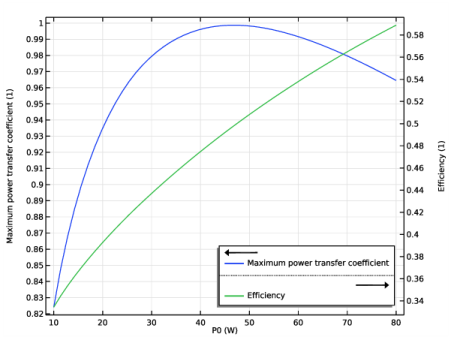
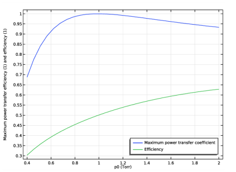
In the Settings window for Global, click Replace Expression in the upper-right corner of the y-Axis Data section. From the menu, choose Component 1 (comp1)>Plasma, Time Periodic>Metal Contact 1>Circuit variables>ptp.mct1.alphaP - Maximum power transfer coefficient.
|
|
3
|
|
1
|
|
2
|
In the Settings window for Global, click Replace Expression in the upper-right corner of the y-Axis Data section. From the menu, choose Component 1 (comp1)>Plasma, Time Periodic>Metal Contact 1>Circuit variables>ptp.mct1.etaP - Efficiency.
|
|
1
|
|
2
|
|
3
|
|
4
|
|
5
|
|
6
|
|
7
|
|
8
|