PDF

Inductively Coupled Plasma (ICP) Torch
Introduction
Thermal plasmas have nowadays a large range of industrial applications including cutting, welding, spraying, waste destruction, and surface treatment. Thermal plasmas are assumed to be under partial to complete local thermodynamic equilibrium (LTE) conditions. Under LTE, the plasma can be considered a conductive fluid mixture and therefore, be modeled using the magnetohydrodynamics (MHD) equations. This model shows how to use the Equilibrium Inductively Coupled Discharge interface to simulate the plasma generated in an inductively coupled plasma torch.
Figure 1 displays the geometry of the to-be-modeled inductive plasma torch.
Figure 1: Geometry of an inductively coupled plasma torch. The torch is composed of three concentric quartz tubes in which gas are injected from the bottom and exit from the top the torch. In this model, a fixed power of 11 kW is transferred to the plasma by a three-turn coil operating at 3MHz.
Note: This application requires the Plasma Module and AC/DC Module.
Model Definition
This model is based on the work presented in Ref. 1 and uses the following assumptions:
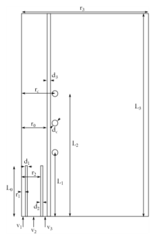
Figure 2 shows the geometry of the model.
Figure 2: Schematic of the ICP torch. Flow enters from the base (v1, v2 and v3) and leaves out the top. The dimensions of the different part of the model are given in the Modeling Instructions section.
In this model excitation is provided to a three turns coil at 3 MHz. The gas flowing in the sheath tube (plasma confinement tube) is then ionized by Joule heating.
The model is solved using a frequency-transient study in combination with a single turn coil feature which set a fixed power to the system (11 kW). By fixing the power, the current and electric potential can vary in the coil as the plasma electrical conductivity builds up. Steady state is reached when the coil current stabilized to its nominal value.
In this model the three different gas stream velocities (v1 for the carrier tube, v2 for the central tube and v3 for the sheath tube) are composed of pure argon. The temperature-dependent physical properties of argon are loaded from the material library under Equilibrium Discharge. Note that the temperature range of the physical properties span from 500 K to 25,000K. Note also that a minimum electrical conductivity has been used to initiate the plasma. The latter has been set to 1 S/m.
Results and Discussion
Figure 3 and Figure 4, respectively, shows the plasma temperature distribution and velocity magnitude of the argon plasma after 0.3 s. Figure 5 shows the electrical conductivity of the plasma at the same time (0.3 s). Note that, for this figure, the electrical conductivity of the other constituents of the model has been set to 0 for sake of visualization.
Figure 6 displays the magnetic flux norm at steady state (0.3 s). Note that the electrical conductivity of the plasma screens the magnetic flux as a consequence of the skin effect.
Figure 7 shows the coil current as a function of the simulation time. The steady state is reached when the current stabilizes (around t = 0.3 s).
Figure 3: Surface plot of the LTE plasma temperature.
Figure 4: Plot of the velocity magnitude.
Figure 5: Plot of the plasma electrical conductivity.
Figure 6: Norm of the magnetic flux. Note the effect of the resistivity on the penetration of the field (skin effect).
Figure 7: Coil current as a function of time for a fixed excitation power. Note the stabilization of the current density as the system reach the steady state.
Reference
1. S. Xue, P. Proulx, and M.I. Boulos, “Extended-field electromagnetic model for inductively coupled plasma,” J. Phys. D. 34, 1897, 2001.
Application Library path: Plasma_Module/Equilibrium_Discharges/icp_torch
Modeling Instructions
From the File menu, choose New.
New
In the New window, click  Model Wizard.
Model Wizard
1
In the Model Wizard window, click  2D Axisymmetric.
2
In the Select Physics tree, select Plasma>Equilibrium Discharges>Equilibrium Inductively Coupled Plasma.
3
Click Add.
4
Click  Study.
5
In the Select Study tree, select Preset Studies for Selected Multiphysics>Frequency-Transient.
6
Root
Select the mm units.
Geometry 1
1
In the Model Builder window, under Component 1 (comp1) click Geometry 1.
2
In the Settings window for Geometry, locate the Units section.
3
From the Length unit list, choose mm.
Global Definitions
Parameters 1
1
In the Model Builder window, under Global Definitions click Parameters 1.
2
In the Settings window for Parameters, locate the Parameters section.
3
Define the computational domain.
Geometry 1
Rectangle 1 (r1)
1
In the Geometry toolbar, click  Rectangle.
2
In the Settings window for Rectangle, locate the Size and Shape section.
3
In the Width text field, type r_3.
4
In the Height text field, type L_3.
Define the carrier tube.
Rectangle 2 (r2)
1
In the Geometry toolbar, click  Rectangle.
2
In the Settings window for Rectangle, locate the Size and Shape section.
3
In the Width text field, type d_1.
4
In the Height text field, type L_0.
5
Locate the Position section. In the r text field, type r_1.
Define the central tube.
Rectangle 3 (r3)
1
In the Geometry toolbar, click  Rectangle.
2
In the Settings window for Rectangle, locate the Size and Shape section.
3
In the Width text field, type d_2.
4
In the Height text field, type L_0.
5
Locate the Position section. In the r text field, type r_2.
Define the tube.
Rectangle 4 (r4)
1
In the Geometry toolbar, click  Rectangle.
2
In the Settings window for Rectangle, locate the Size and Shape section.
3
In the Width text field, type d_3.
4
In the Height text field, type L_3.
5
Locate the Position section. In the r text field, type r_0.
Define the coils.
Circle 1 (c1)
1
In the Geometry toolbar, click  Circle.
2
In the Settings window for Circle, locate the Size and Shape section.
3
In the Radius text field, type d_c/2.
4
Locate the Position section. In the r text field, type r_c.
5
In the z text field, type L_1.
Circle 2 (c2)
1
In the Geometry toolbar, click  Circle.
2
In the Settings window for Circle, locate the Size and Shape section.
3
In the Radius text field, type d_c/2.
4
Locate the Position section. In the r text field, type r_c.
5
In the z text field, type (L_1+L_2)/2.
Circle 3 (c3)
1
In the Geometry toolbar, click  Circle.
2
In the Settings window for Circle, locate the Size and Shape section.
3
In the Radius text field, type d_c/2.
4
Locate the Position section. In the r text field, type r_c.
5
In the z text field, type L_2.
6
Click  Build All Objects.
Define the different domain type for easy selection.
Definitions
Air
1
In the Definitions toolbar, click  Explicit.
2
Right-click Explicit 1 and choose Rename.
3
In the Rename Explicit dialog box, type Air in the New label text field.
4
5
Plasma
1
In the Definitions toolbar, click  Explicit.
2
In the Model Builder window, right-click Explicit 2 and choose Rename.
3
In the Rename Explicit dialog box, type Plasma in the New label text field.
4
5
Quartz
1
In the Definitions toolbar, click  Explicit.
2
Right-click Explicit 3 and choose Rename.
3
In the Rename Explicit dialog box, type Quartz in the New label text field.
4
5
Coils
1
In the Definitions toolbar, click  Explicit.
2
In the Model Builder window, right-click Explicit 4 and choose Rename.
3
In the Rename Explicit dialog box, type Coils in the New label text field.
4
5
Add the different materials used in the model using the material library.
Add Material
1
In the Home toolbar, click  Add Material to open the Add Material window.
2
Go to the Add Material window.
3
4
Click Add to Component in the window toolbar.
5
6
Click Add to Component in the window toolbar.
7
8
Click Add to Component in the window toolbar.
9
In the tree, select Equilibrium Discharge>Argon.
10
Click Add to Component in the window toolbar.
11
In the Home toolbar, click  Add Material to close the Add Material window.
Materials
Air (mat1)
1
In the Model Builder window, under Component 1 (comp1)>Materials click Air (mat1).
2
In the Settings window for Material, locate the Geometric Entity Selection section.
3
From the Selection list, choose Air.
Copper (mat2)
1
In the Model Builder window, click Copper (mat2).
2
In the Settings window for Material, locate the Geometric Entity Selection section.
3
From the Selection list, choose Coils.
Quartz (mat3)
1
In the Model Builder window, click Quartz (mat3).
2
In the Settings window for Material, locate the Geometric Entity Selection section.
3
From the Selection list, choose Quartz.
Argon (mat4)
1
In the Model Builder window, click Argon (mat4).
2
In the Settings window for Material, locate the Geometric Entity Selection section.
3
From the Selection list, choose Plasma.
Adjust the selection and features of each physics composing the model.
The magnetic field interface is used over the whole computational domain. The Single conductor Coil feature is used here to transfer the excitation power to the plasma.
Magnetic Fields (mf)
1
In the Model Builder window, under Component 1 (comp1) click Magnetic Fields (mf).
2
In the Settings window for Magnetic Fields, click to expand the Discretization section.
3
From the Magnetic vector potential list, choose Linear.
Coil 1
1
In the Physics toolbar, click  Domains and choose Coil.
2
In the Settings window for Coil, locate the Domain Selection section.
3
From the Selection list, choose Coils.
4
Locate the Coil section. Select the Coil group check box.
5
From the Coil excitation list, choose Power.
6
In the Pcoil text field, type Pext.
The heat transfer in the air is neglected in this model.
Heat Transfer in Fluids (ht)
1
In the Model Builder window, under Component 1 (comp1) click Heat Transfer in Fluids (ht).
2
Solid 1
1
In the Physics toolbar, click  Domains and choose Solid.
2
Initial Values 1
1
In the Model Builder window, click Initial Values 1.
2
In the Settings window for Initial Values, locate the Initial Values section.
3
In the T text field, type T0.
Add a heat transfer in solids feature for the solid part of the heat transfer model (tubes and coils).
Temperature 1
1
In the Physics toolbar, click  Boundaries and choose Temperature.
2
3
In the Settings window for Temperature, locate the Temperature section.
4
In the T0 text field, type T0.
Outflow 1
1
In the Physics toolbar, click  Boundaries and choose Outflow.
2
Click the  Zoom Extents button in the Graphics toolbar.
3
The single phase flow is only applied to the plasma.
Laminar Flow (spf)
Since the density variation is not small, the flow cannot be regarded as incompressible. Therefore set the flow to be weakly compressible. Add some isotropic diffusion which is initially very high then ramps down to zero after the plasma has ignited.
1
In the Model Builder window, under Component 1 (comp1) click Laminar Flow (spf).
2
In the Settings window for Laminar Flow, locate the Physical Model section.
3
From the Compressibility list, choose Weakly compressible flow.
4
Locate the Domain Selection section. From the Selection list, choose Plasma.
5
Click to expand the Equation section. From the Equation form list, choose Stationary.
6
Click the  Show More Options button in the Model Builder toolbar.
7
In the Show More Options dialog box, in the tree, select the check box for the node Physics>Stabilization.
8
9
In the Model Builder window, click Laminar Flow (spf).
10
In the Settings window for Laminar Flow, click to expand the Inconsistent Stabilization section.
11
Find the Navier-Stokes equations subsection. Select the Isotropic diffusion check box.
12
In the δid text field, type 2*(1-tanh(100*(t[1/s]-0.08))).
Since the equation form for laminar flow is stationary and the study to resolve is frequency-transient, deactivate the Pseudo-time-stepping in Advanced settings.
13
Click the  Show More Options button in the Model Builder toolbar.
14
In the Show More Options dialog box, in the tree, select the check box for the node Physics>Advanced Physics Options.
15
16
In the Settings window for Laminar Flow, click to expand the Advanced Settings section.
17
Find the Pseudo time stepping subsection. From the Use pseudo time stepping for stationary equation form list, choose Off.
Inlet 1
1
In the Physics toolbar, click  Boundaries and choose Inlet.
Add the inlets with their proper velocities.
2
3
In the Settings window for Inlet, locate the Velocity section.
4
In the U0 text field, type v1.
Inlet 2
1
In the Physics toolbar, click  Boundaries and choose Inlet.
2
3
In the Settings window for Inlet, locate the Velocity section.
4
In the U0 text field, type v2.
Inlet 3
1
In the Physics toolbar, click  Boundaries and choose Inlet.
2
3
In the Settings window for Inlet, locate the Velocity section.
4
In the U0 text field, type v3.
Outlet 1
1
In the Physics toolbar, click  Boundaries and choose Outlet.
2
3
In the Settings window for Outlet, locate the Pressure Conditions section.
4
Clear the Suppress backflow check box.
Mesh 1
Size
In the Model Builder window, under Component 1 (comp1) right-click Mesh 1 and choose Edit Physics-Induced Sequence.
Size 1
1
In the Settings window for Size, locate the Element Size section.
2
From the Predefined list, choose Extra fine.
Edge 1
1
In the Mesh toolbar, click  Edge.
2
Size 1
1
Right-click Edge 1 and choose Size.
2
In the Settings window for Size, locate the Element Size section.
3
Click the Custom button.
4
Click to collapse the Element Size Parameters section. Click to expand the Element Size Parameters section. Select the Maximum element size check box.
5
Size 2
1
In the Model Builder window, click Size 2.
2
In the Settings window for Size, locate the Element Size section.
3
From the Predefined list, choose Extra fine.
Boundary Layers 2
1
In the Mesh toolbar, click  Boundary Layers.
2
Right-click Boundary Layers 2 and choose Move Up.
3
In the Settings window for Boundary Layers, locate the Domain Selection section.
4
From the Geometric entity level list, choose Domain.
5
Boundary Layer Properties
1
In the Model Builder window, click Boundary Layer Properties.
2
3
In the Settings window for Boundary Layer Properties, locate the Boundary Layer Properties section.
4
In the Number of boundary layers text field, type 4.
5
From the Thickness of first layer list, choose Manual.
6
In the Thickness text field, type 8[um].
7
Click  Build All.
Study 1
1
In the Model Builder window, click Study 1.
2
In the Settings window for Study, locate the Study Settings section.
3
Clear the Generate default plots check box.
Solution 1 (sol1)
In the Study toolbar, click  Show Default Solver.
Step 1: Frequency-Transient
1
In the Model Builder window, click Step 1: Frequency-Transient.
2
In the Settings window for Frequency-Transient, locate the Study Settings section.
3
In the Output times text field, type range(0,0.05,1)*0.3.
4
In the Frequency text field, type freq.
Solver Configurations
In the Model Builder window, expand the Study 1>Solver Configurations node.
Solution 1 (sol1)
1
In the Model Builder window, expand the Study 1>Solver Configurations>Solution 1 (sol1)>Time-Dependent Solver 1>Segregated 1 node, then click Velocity u, Pressure p.
2
In the Settings window for Segregated Step, click to expand the Method and Termination section.
3
From the Jacobian update list, choose On every iteration.
To improve the robustness of the solver, add temperature to the segregated step of velocity and pressure.
4
Locate the General section. Under Variables, click  Add.
5
In the Add dialog box, select Temperature (comp1.T) in the Variables list.
6
7
In the Settings window for Segregated Step, type Velocity u, Pressure p, Temperature T in the Label text field.
8
In the Model Builder window, right-click Temperature and choose Disable.
9
Right-click Magnetic Fields and choose Move Down.
10
In the Study toolbar, click  Compute.
Create some relevant figures.
The temperature.
Results
Temperature
1
In the Home toolbar, click  Add Plot Group and choose 2D Plot Group.
2
Right-click 2D Plot Group 1 and choose Rename.
3
In the Rename 2D Plot Group dialog box, type Temperature in the New label text field.
4
Surface 1
1
Right-click Temperature and choose Surface.
2
In the Settings window for Surface, locate the Expression section.
3
In the Expression text field, type T.
4
In the Temperature toolbar, click  Plot.
Duplicate the figure to display the fluid velocity magnitude.
Velocity
1
In the Model Builder window, right-click Temperature and choose Duplicate.
2
Right-click Temperature 1 and choose Rename.
3
In the Rename 2D Plot Group dialog box, type Velocity in the New label text field.
4
Surface 1
1
In the Model Builder window, expand the Velocity node, then click Surface 1.
2
In the Settings window for Surface, locate the Expression section.
3
In the Expression text field, type spf.U.
4
In the Velocity toolbar, click  Plot.
Duplicate the figure to display the electrical conductivity.
Electrical conductivity
1
In the Model Builder window, right-click Velocity and choose Duplicate.
2
Right-click Velocity 1 and choose Rename.
3
In the Rename 2D Plot Group dialog box, type Electrical conductivity in the New label text field.
4
Surface 1
1
In the Model Builder window, expand the Electrical conductivity node, then click Surface 1.
2
In the Settings window for Surface, locate the Expression section.
3
In the Expression text field, type mf.sigmarr*(dom==1).
4
In the Electrical conductivity toolbar, click  Plot.
Duplicate the figure to display the norm of the magnetic flux. Note the effect of the plasma conductivity on the skin depth.
Magnetic flux
1
In the Model Builder window, right-click Electrical conductivity and choose Duplicate.
2
Right-click Electrical conductivity 1 and choose Rename.
3
In the Rename 2D Plot Group dialog box, type Magnetic flux in the New label text field.
4
Surface 1
1
In the Model Builder window, expand the Magnetic flux node, then click Surface 1.
2
In the Settings window for Surface, locate the Expression section.
3
In the Expression text field, type mf.normB.
4
In the Magnetic flux toolbar, click  Plot.
Display the coil current as a function of time. Note the time it takes to get the steady state (constant current in the coils).
Coil current
1
In the Home toolbar, click  Add Plot Group and choose 1D Plot Group.
2
Right-click 1D Plot Group 5 and choose Rename.
3
In the Rename 1D Plot Group dialog box, type Coil current in the New label text field.
4
Global 1
1
Right-click Coil current and choose Global.
2
In the Settings window for Global, locate the y-Axis Data section.
3
4
In the Coil current toolbar, click  Plot.
Create a nice 3D plot for the model thumbnail.
Create first a revolution dataset.
Revolution 2D 1
1
In the Results toolbar, click  More Datasets and choose Revolution 2D.
2
In the Settings window for Revolution 2D, click to expand the Revolution Layers section.
3
In the Start angle text field, type -90.
4
In the Revolution angle text field, type 225.
Then create the 3D plot.
Temperature 3D
1
In the Results toolbar, click  3D Plot Group.
2
Right-click 3D Plot Group 6 and choose Rename.
3
In the Rename 3D Plot Group dialog box, type Temperature 3D in the New label text field.
4
Volume 1
1
Right-click Temperature 3D and choose Volume.
2
In the Settings window for Volume, locate the Expression section.
3
In the Expression text field, type T.
4
In the Temperature 3D toolbar, click  Plot.
5
Click the  Go to Default View button in the Graphics toolbar.
Set the figure as a model thumbnail by clicking on the root folder in the model builder than expand the model thumbnail section and click on set model thumbnail.