PDF

Drift Diffusion Tutorial
Introduction
The foundation of the COMSOL Multiphysics Plasma Module is the Drift Diffusion interface, which describes the transport of electrons in an electric field. The Drift Diffusion interface solves a pair of reaction/convection/diffusion equations, one for the electron density and the other for the electron energy density. The mean electron energy is computed by dividing the electron energy density by the electron number density.
Model Definition
This tutorial example computes the electron number density and mean electron energy in a drift tube. Electrons are released due to thermionic emission on the left boundary with an assumed mean electron energy. The electrons are then accelerated toward the right boundary due to an imposed external electric field that is oriented in the opposite direction from the electron drift velocity:
Figure 1: In the drift tube the electrons enter the left boundary and are accelerated by the electric field toward the wall.
model equations
A simple model is set up to test the Drift Diffusion interface. The equations solved are, for the electron number density:
(1)
where
(2)
and, ne denotes the electron density (1/m3), Re is the electron rate expression (1/(m3·s)), μe is the electron mobility which is either a scalar or tensor (m2/(V·s)), E is the electric field (V/m), and De is the electron diffusivity, which is either a scalar or a tensor. The first term on the right side of Equation 2 represents migration of electrons due to an electric field. The second term on the right side of Equation 2 represents diffusion of electrons from regions of high electron density to low electron density.
An equation for the electron energy density is solved in conjunction with Equation 1. The equation is:
(3)
where
Here, nε is the electron energy density (V/m3), Rε is the energy loss/gain due to inelastic collisions (V/(m3·s)), με is the electron energy mobility (m2/(V·s)), E is the electric field (V/m), and Dε is the electron energy diffusivity (m2/s). The subscript ε refers to electron energy. The third term on the left side of Equation 3 represents heating of the electrons due to an external electric field. Note that this term can either be a heat source or a heat sink depending on whether the electrons are drifting in the same direction as the electric field or not. For a Maxwellian electron energy distribution function, the following relationships hold:
where Te is the electron “temperature”. So, given the electron mobility, the other transport properties required can be computed. The electron “temperature” is a function of the mean electron energy, , which is defined as:
and then:
source coefficients
The electron source term, Re is the sum of the electron impact reaction rates that make up the plasma chemistry. The electron energy loss due to inelastic collisions, Rε is a function of the electron impact reaction rates multiplied by the energy loss corresponding to each reaction. Mathematically, the electron source is defined as:
where xj is the mole fraction of the target species for reaction j, kj is the rate coefficient for reaction j (m3/s), and Nn is the total neutral number density (1/m3). The energy loss is defined as:
where Δεj is the energy loss from reaction j (V).
An influx of electron due to thermionic emission is specified on the left boundary. The electrons that are emitted from the surface are then accelerated toward the wall by the electric field. The acceleration leads to an increase in the mean electron energy and subsequently ionization occurs. This creates new electrons, which are ultimately lost into a wall opposite the emitting surface. The gain of electrons due to ionization is included in the model by assuming the drift tube contains argon. This example assumes that the mole fraction of electronically excited argon atoms and argon ions is very small. This means that you do not solve additional equations for the mole fractions of these two species. The following reactions are included in the model:
The rate constants for these reactions are given in Arrhenius form:
The rate constants are computed from cross-section data for each reaction assuming a Maxwellian electron energy distribution function.
Results and Discussion
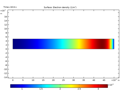
The electron density is plotted in Figure 2. The peak electron density occurs close to the far wall. The peak electron density is five times higher than the electron density on the left wall due to new electrons being created through ionization.
Figure 2: Plot of the electron density in the drift tube.
Because there are no variations in the solution in the y-direction it can be more convenient to create a 1D data set in the x-direction and plot various quantities versus the x-axis. Figure 3 plots the electron density as a function of the x-direction. The electron “temperature” is plotted in Figure 4. On the left wall the electron “temperature” is fixed to 2 eV. The temperature steadily increases over a narrow region. This is because there is a strong drift velocity in the opposite direction to the electric field. As the electron temperature increases, so do the rate constants, which are responsible for creating new electrons. The increase in electron temperature also has a significant effect on the number of inelastic collisions that occur in the tube. After the initial rise in electron temperature, the electron temperature remains constant until close to the far wall. In this region the Joule heating caused by the electron drift velocity in the opposite direction to the electric field is balanced by the energy loss due to inelastic collisions.
The highly nonlinear behavior in such a simple example showcases the fact that very complicated dynamics occur in even the simplest of plasmas.
Figure 3: Plot of the electron “temperature” across the drift tube.
Figure 4: Cross section plot of electron density across the drift tube.
Figure 5: Cross plot of the electron temperature across the drift tube.
Reference
1. G.J.M. Hagelaar and L.C. Pitchford, “Solving the Boltzmann equation to obtain electron transport coefficients and rate coefficients for fluid models,” Plasma Sources Sci. Technol., vol. 14, pp. 722–733, 2005.
Application Library path: Plasma_Module/Direct_Current_Discharges/drift_diffusion_tutorial
Modeling Instructions
From the File menu, choose New.
New
In the New window, click  Model Wizard.
Model Wizard
1
In the Model Wizard window, click  2D.
2
In the Select Physics tree, select Plasma>Species Transport>Drift Diffusion (dd).
3
Click Add.
4
Click  Study.
5
In the Select Study tree, select General Studies>Time Dependent.
6
Geometry 1
Rectangle 1 (r1)
1
In the Geometry toolbar, click  Rectangle.
2
In the Settings window for Rectangle, locate the Size and Shape section.
3
In the Width text field, type 5E-3.
4
In the Height text field, type 5E-4.
Now add a table of expressions for the external electric field, temperature, pressure, and the electron impact reactions occurring in the drift tube. You also define the influx of electrons due to thermionic emission. The influx of electrons and the external electric field are both ramped up from an initial value of zero to aid convergence at early timesteps.
Definitions
Variables 1
1
In the Home toolbar, click  Variables and choose Local Variables.
2
In the Settings window for Variables, locate the Variables section.
3
Drift Diffusion (dd)
1
In the Model Builder window, under Component 1 (comp1) click Drift Diffusion (dd).
2
In the Settings window for Drift Diffusion, locate the Electron Properties section.
3
Select the Use reduced electron transport properties check box.
Drift Diffusion Model 1
1
In the Model Builder window, under Component 1 (comp1)>Drift Diffusion (dd) click Drift Diffusion Model 1.
2
In the Settings window for Drift Diffusion Model, locate the Model Inputs section.
3
In the Nn text field, type Nn0.
4
In the V text field, type V.
5
In the Sen text field, type Sen.
6
Locate the Electron Density and Energy section. In the μeNn text field, type mueN.
Initial Values 1
1
In the Model Builder window, click Initial Values 1.
2
In the Settings window for Initial Values, locate the Initial Values section.
3
In the ne,0 text field, type 1E16.
4
In the ε0 text field, type 3.
Electron Production Rate 1
1
In the Physics toolbar, click  Domains and choose Electron Production Rate.
2
3
In the Settings window for Electron Production Rate, locate the Electron Production Rate section.
4
In the Re text field, type Re.
Wall 1
1
In the Physics toolbar, click  Boundaries and choose Wall.
2
In the Settings window for Wall, locate the General Wall Settings section.
3
Select the Include migration effects check box.
4
Electron Density and Energy 1
1
In the Physics toolbar, click  Boundaries and choose Electron Density and Energy.
2
3
In the Settings window for Electron Density and Energy, locate the Electron Density and Energy section.
4
Select the Fix mean electron energy check box.
Wall 2
1
In the Physics toolbar, click  Boundaries and choose Wall.
2
3
In the Settings window for Wall, locate the Electron Density Wall Settings section.
4
In the Γt·n text field, type influx.
5
Locate the Electron Energy Wall Settings section. Clear the Use wall for electron energy check box.
The above boundary conditions applied to boundary 1 means that the mean electron energy will be fixed at 3 electron volts and there will be an influx of electrons resulting in a net current influx of 2E-6 amps.
When you create the mesh you want to use a finer mesh close to the walls so that the sharp gradients in the electron density and electron energy density are adequately resolved. You accomplish this by using a graded mapped mesh.
Mesh 1
Mapped 1
In the Model Builder window, under Component 1 (comp1) right-click Mesh 1 and choose Mapped.
Distribution 1
1
In the Model Builder window, right-click Mapped 1 and choose Distribution.
2
3
In the Settings window for Distribution, locate the Distribution section.
4
From the Distribution type list, choose Predefined.
5
In the Number of elements text field, type 200.
6
In the Element ratio text field, type 5.
7
From the Growth formula list, choose Geometric sequence.
8
Select the Symmetric distribution check box.
Size
1
In the Model Builder window, click Size.
2
In the Settings window for Size, locate the Element Size section.
3
From the Predefined list, choose Extra fine.
4
Click  Build All.
The mean electron energy and electron density can change on a subnanosecond time scale. The electron density and mean electron energy reach their steady state values very quickly so it is only necessary to solve the problem for 1 microsecond.
Study 1
Step 1: Time Dependent
1
In the Model Builder window, under Study 1 click Step 1: Time Dependent.
2
In the Settings window for Time Dependent, locate the Study Settings section.
3
In the Output times text field, type 0.
4
Click  Range.
5
In the Range dialog box, choose Number of values from the Entry method list.
6
In the Start text field, type -8.
7
In the Stop text field, type -6.
8
In the Number of values text field, type 100.
9
From the Function to apply to all values list, choose exp10(x) – Exponential function (base 10).
10
Click Add.
11
In the Home toolbar, click  Compute.
Results
Electron Density (dd)
1
In the Settings window for 2D Plot Group, click to expand the Window Settings section.
2
Locate the Color Legend section. From the Position list, choose Bottom.
3
Click the  Zoom Extents button in the Graphics toolbar.
4
In the Electron Density (dd) toolbar, click  Plot.
Electron Temperature (dd)
1
In the Model Builder window, click Electron Temperature (dd).
2
In the Settings window for 2D Plot Group, locate the Color Legend section.
3
From the Position list, choose Bottom.
4
Click the  Zoom Extents button in the Graphics toolbar.
5
In the Electron Temperature (dd) toolbar, click  Plot.
Cut Line 2D 1
1
In the Results toolbar, click  Cut Line 2D.
2
Click the  Zoom Extents button in the Graphics toolbar.
3
In the Settings window for Cut Line 2D, locate the Line Data section.
4
In row Point 1, set Y to 2.5e-4.
5
In row Point 2, set Y to 2.5e-4 and x to 5-3.
6
1D Plot Group 3
1
In the Results toolbar, click  1D Plot Group.
2
In the Settings window for 1D Plot Group, locate the Data section.
3
From the Dataset list, choose Cut Line 2D 1.
4
From the Time selection list, choose Last.
Line Graph 1
1
Right-click 1D Plot Group 3 and choose Line Graph.
2
In the Settings window for Line Graph, click Replace Expression in the upper-right corner of the y-axis data section. From the menu, choose Component 1 (comp1)>Drift Diffusion>Electron density>dd.ne - Electron density - 1/m³.
3
In the 1D Plot Group 3 toolbar, click  Plot.
1D Plot Group 4
1
In the Home toolbar, click  Add Plot Group and choose 1D Plot Group.
2
In the Settings window for 1D Plot Group, locate the Data section.
3
From the Dataset list, choose Cut Line 2D 1.
4
From the Time selection list, choose Last.
Line Graph 1
1
Right-click 1D Plot Group 4 and choose Line Graph.
2
In the Settings window for Line Graph, click Replace Expression in the upper-right corner of the y-axis data section. From the menu, choose Component 1 (comp1)>Drift Diffusion>Electron energy density>dd.Te - Electron temperature - V.
3
In the 1D Plot Group 4 toolbar, click  Plot.