PDF

Electrical Breakdown Between Spheres
Introduction
Whether electrical breakdown will occur in an electrical system depends on a number of parameters including geometry, applied voltage, fill gas, pressure and temperature. A fully self consistent plasma model of an electrical system can be very tricky, especially if the geometry is complicated. It is possible to estimate whether electrical breakdown will occur without solving a full blown plasma model, by integrating Townsend growth coefficients along electric field lines. This model shows how to do this for electrical breakdown between two spheres.
Model Definition
This tutorial example shows that the onset of electrical breakdown between two spheres separated by 2 cm, will occur at 51.8 kV for dry air at room temperature.The Electrical Breakdown Detection interface defines 3 different regimes which can occur in any given device. The breakdown condition for a self-sustaining discharge is given by the following:
(1)
where γi is the secondary emission coefficient (dimensionless), N is the number density (SI unit: 1/m3), α is the reduced Townsend growth/decay coefficient (SI unit: m2), s is the arc length along the particle trajectory, and D is the distance from the source boundary to any destination boundary. Using this, the following 3 regimes are defined.
No discharge
Re–arranging Equation 1, it is obvious that no discharge will occur if the following condition is true:
(2).
sustained Discharge
When the left hand side of Equation 1 is greater than 1, a self–sustaining discharge can occur. Another way of writing this condition is that a self sustained discharge can form when the Townsend condition is met:
(3).
This isn’t necessarily catastrophic to an electrical design, since the current is usually limited in such a discharge. The third case however, can be catastrophic.
streamer
When the exponential of the left hand side is above around 108, a streamer will form across the gap. Mathematically, the streamer condition is given by:
(4)
where d is the gap distance in cm.
The Electrical Breakdown Detection physics interface defines a variable, ebd.bi which takes the value of 0 for the no discharge case, 1 for the sustained discharge and 2 for the streamer. This variable is plotted by default when running a study.
All the information about which regime the system will operate is embedded in the reduced Townsend coefficient, α. The reduced Townsend coefficient is a strong function of the reduced electric field:
(5)
where E is the electric field parallel to the streamlines (SI unit: V/m). The software computes the integral by solving an ordinary differential equation along the test particle trajectories:
(6)
where Nstp is the number density at standard temperature and pressure. Another quantity of interest is the pressure multiplied by the path length. This is also computed by solving the following ordinary differential equation:
(7)
where it is assumed the pressure is constant along the trajectory.
In this model, the Townsend growth coefficient is taken using the Dry air option, which uses an interpolation function for the growth coefficient vs. reduced electric field, from Ref. 2.
Results and Discussion
The electric field from the electrostatic study is shown in Figure 1. As expected, the electric field is strongest at the minimum distance between the two spheres. Any seed electrons exposed to this electric field have the potential to gain enough energy to ionize the background gas, possibly setting off a positive feedback loop whereby an electron avalanche can occur.
Figure 1: Plot of the electric field between two spheres.
The breakdown indicator for this configuration is shown in Figure 2 below. When the indicator is zero, no discharge will occur, when the indicator is one, a (current limited) Townsend discharge may occur. Since this is current limited, it is not necessarily a problem in the electrical system. However, when the indicator is two, as shown by the small red spot on the left sphere (at the minimum distance between the two spheres), a streamer may form which is not current limited, which can potentially be catastrophic to an electrical system. As expected, the region for streamer formation is a very small dot, meaning that onset is only just occurring. This is expected, since the applied voltage is right at the value (51.8 kV) where this should be the case.
Figure 2: Electrical breakdown indicator on the cathode surface.
The integrated Townsend growth coefficient is show in Figure 3. When this is above around 18.3, streamer formation can occur. There is a substantial variation in this function over the cathode – away from the minimum distance between the two spheres, the integrated growth coefficient is substantially under the streamer threshold.
Figure 3: Integrated Townsend growth coefficient on the cathode surface. Once this value gets above around 18, electrical breakdown will occur.
Finally, in Figure 4 the pressure times the path length is plotted in units of torr-cm. This quantity can be of interest, since Paschen curves usually plot the breakdown voltage vs. pressure times gap. Providing this as a default plot makes it easy to verify that breakdown is occurring at the expected voltage (for a given pressure times gap length), since experimental Paschen curve data is often available.
Figure 4: Plot of the pressure times the path length, in units of torr cm. The values are within the range in which the approximate method used to detect electrical breakdown is valid.
Reference
1. Larry K. Warne, Roy E. Jorgenson and Scott D. Nicolaysen, Ionization Coefficient Approach to Modeling Breakdown in Nonuniform Geometries, Sandia Report (2003).
2. J. Dutton, A survey of Electron Swarm Data, J. Phys. Chem. Ref. Data, Vol 4, No 3, 1975.
Application Library path: Plasma_Module/Electrical_Breakdown_Detection/breakdown_between_spheres
Modeling Instructions
From the File menu, choose New.
New
In the New window, click  Model Wizard.
Model Wizard
1
In the Model Wizard window, click  3D.
2
In the Select Physics tree, select AC/DC>Electric Fields and Currents>Electrostatics (es).
3
Click Add.
4
Click  Study.
5
In the Select Study tree, select General Studies>Stationary.
6
Global Definitions
Parameters 1
1
In the Model Builder window, under Global Definitions click Parameters 1.
2
In the Settings window for Parameters, locate the Parameters section.
3
Geometry 1
Sphere 1 (sph1)
1
In the Model Builder window, expand the Component 1 (comp1)>Geometry 1 node.
2
Right-click Geometry 1 and choose Sphere.
3
In the Settings window for Sphere, locate the Size section.
4
In the Radius text field, type a.
5
Locate the Rotation Angle section. In the Rotation text field, type 45.
Rotate 1 (rot1)
1
In the Geometry toolbar, click  Transforms and choose Rotate.
2
3
In the Settings window for Rotate, locate the Rotation section.
4
From the Axis type list, choose Cartesian.
5
In the y text field, type 1.
6
In the z text field, type 0.
7
In the Angle text field, type 45.
8
Click  Build All Objects.
Sphere 2 (sph2)
1
In the Geometry toolbar, click  Sphere.
2
In the Settings window for Sphere, locate the Size section.
3
In the Radius text field, type a.
4
Locate the Position section. In the x text field, type 2*hg.
Block 1 (blk1)
1
In the Geometry toolbar, click  Block.
2
In the Settings window for Block, locate the Size and Shape section.
3
In the Width text field, type 20[cm].
4
In the Depth text field, type 20[cm].
5
In the Height text field, type 20[cm].
6
Locate the Position section. In the x text field, type -8[cm].
7
In the y text field, type -10[cm].
8
In the z text field, type -10[cm].
9
Click  Build All Objects.
10
Click the  Go to Default View button in the Graphics toolbar.
11
Click the  Wireframe Rendering button in the Graphics toolbar.
Difference 1 (dif1)
1
In the Geometry toolbar, click  Booleans and Partitions and choose Difference.
2
3
In the Settings window for Difference, locate the Difference section.
4
Find the Objects to subtract subsection. Select the  Activate Selection toggle button.
5
Select the objects rot1 and sph2 only.
6
Click  Build All Objects.
Materials
Material 1 (mat1)
1
In the Model Builder window, under Component 1 (comp1) right-click Materials and choose Blank Material.
2
In the Settings window for Material, locate the Material Contents section.
3
Electrostatics (es)
Ground 1
1
In the Model Builder window, under Component 1 (comp1) right-click Electrostatics (es) and choose Ground.
2
Click the  Select Box button in the Graphics toolbar.
3
Electric Potential 1
1
In the Physics toolbar, click  Boundaries and choose Electric Potential.
2
Click the  Select Box button in the Graphics toolbar.
3
4
In the Settings window for Electric Potential, locate the Electric Potential section.
5
In the V0 text field, type Vapp.
Mesh 1
Size 1
1
In the Model Builder window, under Component 1 (comp1) right-click Mesh 1 and choose Size.
2
In the Settings window for Size, locate the Geometric Entity Selection section.
3
From the Geometric entity level list, choose Boundary.
4
Click the  Select Box button in the Graphics toolbar.
5
6
Click the  Select Box button in the Graphics toolbar.
7
8
Click the  Select Box button in the Graphics toolbar.
9
10
Locate the Element Size section. Click the Custom button.
11
Click to collapse the Element Size Parameters section. Click to expand the Element Size Parameters section. Select the Maximum element size check box.
12
13
Locate the Geometric Entity Selection section. Click  Copy Selection.
Free Triangular 1
1
In the Mesh toolbar, click  Boundary and choose Free Triangular.
2
In the Settings window for Free Triangular, locate the Boundary Selection section.
3
Click  Paste Selection.
4
In the Paste Selection dialog box, type 6-17 in the Selection text field.
5
Free Tetrahedral 1
1
In the Mesh toolbar, click  Free Tetrahedral.
2
In the Settings window for Free Tetrahedral, click  Build All.
3
Click the  Go to Default View button in the Graphics toolbar.
Study 1
In the Home toolbar, click  Compute.
Results
Electric Field
1
In the Model Builder window, expand the Results>Electric Potential (es) node, then click Electric Potential (es).
2
In the Settings window for 3D Plot Group, type Electric Field in the Label text field.
Multislice 1
1
In the Model Builder window, click Multislice 1.
2
In the Settings window for Multislice, locate the Multiplane Data section.
3
Find the x-planes subsection. In the Planes text field, type 0.
4
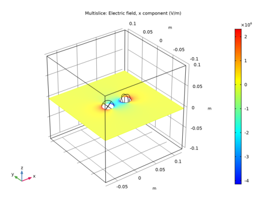
Click Replace Expression in the upper-right corner of the Expression section. From the menu, choose Component 1 (comp1)>Electrostatics>Electric>Electric field - V/m>es.Ex - Electric field, x component.
5
Locate the Multiplane Data section. Find the y-planes subsection. In the Planes text field, type 0.
6
In the Electric Field toolbar, click  Plot.
Add Physics
1
In the Home toolbar, click  Add Physics to open the Add Physics window.
2
Go to the Add Physics window.
3
In the tree, select Plasma>Electrical Breakdown Detection (ebd).
4
Find the Physics interfaces in study subsection. In the table, clear the Solve check box for Study 1.
5
Click Add to Component 1 in the window toolbar.
6
In the Home toolbar, click  Add Physics to close the Add Physics window.
Electrical Breakdown Detection (ebd)
Cathode 1
1
Right-click Component 1 (comp1)>Electrical Breakdown Detection (ebd) and choose Cathode.
2
3
Click the  Go to Default View button in the Graphics toolbar.
Particle Counter 1
1
In the Physics toolbar, click  Boundaries and choose Particle Counter.
2
Electrical Breakdown Detection 1
1
In the Model Builder window, click Electrical Breakdown Detection 1.
2
In the Settings window for Electrical Breakdown Detection, locate the Electric Field section.
3
From the E list, choose Electric field (es/ccn1).
Add Study
1
In the Home toolbar, click  Add Study to open the Add Study window.
2
Go to the Add Study window.
3
Find the Physics interfaces in study subsection. In the table, clear the Solve check box for Electrostatics (es).
4
Find the Studies subsection. In the Select Study tree, select General Studies>Time Dependent.
5
Click Add Study in the window toolbar.
6
In the Home toolbar, click  Add Study to close the Add Study window.
Study 2
Step 1: Time Dependent
1
In the Settings window for Time Dependent, locate the Study Settings section.
2
In the Output times text field, type range(0,0.002,0.15).
3
Click to expand the Values of Dependent Variables section. Find the Values of variables not solved for subsection. From the Settings list, choose User controlled.
4
From the Method list, choose Solution.
5
From the Study list, choose Study 1, Stationary.
6
In the Home toolbar, click  Compute.
Results
Breakdown Indicator (ebd)
1
In the Model Builder window, under Results click Breakdown Indicator (ebd).
2
In the Breakdown Indicator (ebd) toolbar, click  Plot.
Integrated Townsend Growth Coefficient (ebd)
1
In the Model Builder window, click Integrated Townsend Growth Coefficient (ebd).
2
In the Integrated Townsend Growth Coefficient (ebd) toolbar, click  Plot.
Pressure Times Path Length (ebd)
1
In the Model Builder window, click Pressure Times Path Length (ebd).
2
In the Pressure Times Path Length (ebd) toolbar, click  Plot.