PDF

3D ICP Reactor, Argon Chemistry
Introduction
Although not recommended, 3-dimensional plasma modeling is possible to do in COMSOL. A square coil is placed on top of a dielectric window and it electrically excited at 13.56 MHz. A plasma is formed in the chamber beneath the dielectric window, which contains argon gas at low pressure (20 mtorr). The gas flows into the process chamber from two 2 inch ports and the gas is extracted through a single 4 inch port. The plasma is sustained via electromagnetic induction where power is transferred from the electromagnetic fields to the electrons.
Note: This application requires the Plasma Module and the AC/DC Module.
Model Definition
Inductively coupled discharges typically operate at low pressures (<10 Pa) and high charge density (>1017 m3). High density plasma sources are popular because low pressure ion bombardment can provide a greater degree of anisotropy on the surface of the wafer.
Domain equations
The Inductively Coupled Plasma (ICP) reactor interface solves a system of coupled partial differential equations for:
The electron density and mean electron energy are computed by solving a pair of drift-diffusion equations for the electron density and mean electron energy. Convection of electrons due to fluid motion is neglected. For detailed information on electron transport see the Plasma Module User’s Guide.
The electron source Re and the energy loss due to inelastic collisions Rε are defined later. In this model, the electron diffusivity, energy mobility and energy diffusivity are calculated from the electron mobility, μe using:
The source coefficients in the above equations are determined by the plasma chemistry and are written using either rate coefficients. Suppose that there are M reactions which contribute to the growth or decay of electron density and P electron-neutral collisions. In general P >> M. The electron source term is given by
where xj is the mole fraction of the target species for reaction j, kj is the rate coefficient for reaction j (m3/s), and Nn is the total neutral number density (1/m3). The electron energy loss is obtained by summing the collisional energy loss over all reactions:
where Δεj is the energy loss from reaction j (V). The electron source and inelastic energy loss are automatically computed by the Inductively Coupled Plasma interface. The rate coefficients may be computed from cross section data by the following integral:
where γ = (2q/me)1/2 (C1/2/kg1/2), me is the electron mass (kg), ε is energy (V), σk is the collision cross section (m2) and f is the electron energy distribution function (EEDF). In this model a Maxwellian EEDF is assumed.
For non-electron species, the following equation is solved for the mass fraction of each species. For detailed information on the transport of the non-electron species see Theory for the Heavy Species Transport Interface in the Plasma Module User’s Guide.
The electrostatic field is computed using the following equation:
The space charge density ρ is automatically computed based on the plasma chemistry specified in the model using the formula:
For detailed information about electrostatics see Theory for the Electrostatics Interface in the Plasma Module User’s Guide.
For a nonmagnetized, nonpolarized plasma, the induction currents are computed in the frequency domain using the following equation:
The plasma conductivity is automatically defined using the cold plasma approximation:
where ne is the electron density, q is the electron charge, me is the electron mass, νe is the collision frequency and ω is the angular frequency.
plasma chemistry
Since the physics occurring in an inductively coupled plasma is rather complex, it is always best to start a modeling project with a simple chemical mechanism. Argon is one of the simplest mechanisms to implement at low pressures. The electronically excited states can be lumped into a single species which results in a chemical mechanism consisting of only 3 species and 7 reactions (electron impact cross-section are obtained from Ref. 3):
Stepwise ionization (reaction 5) can play an important role in sustaining low pressure argon discharges. Excited argon atoms are consumed via superelastic collisions with electrons, quenching with neutral argon atoms, ionization or Penning ionization where two metastable argon atoms react to form a neutral argon atom, an argon ion and an electron. In addition to volumetric reactions, the following surface reactions are implemented:
When a metastable argon atom makes contact with the wall, it reverts to the ground state argon atom with some probability (the sticking coefficient).
electrical excitation
From an electrical point of view, the GEC reactor behaves as a transformer. A current is applied to the driving coil (the primary) and this induces a current in the plasma (the secondary). The plasma then induces an opposing current back in the coil, increasing its impedance. The current flowing in the plasma depends on the current applied to the coil and the reaction kinetics. The total plasma current may vary from no current (plasma not sustained) to the same current as the primary which corresponds to perfect coupling between the coil and the plasma. Since this is a 3D model it is not practical to resolve the skin depth in the driving coil. Instead an impedance boundary condition is used which only computes the coil current density in the tangential direction of the coil surface. This means the mesh does not have to resolve the skin depth in the coil, which at 13.56MHz for copper is only 17 microns.
Results and Discussion
The peak electron density occurs at the center of the reactor, underneath the RF coil. The electron density in this case is high enough to cause some shielding of the azimuthal electric field.
Figure 1: Plot of electron temperature (slice), magnetic vector potential (streamlines) and electric field norm (streamline color).
The electron “temperature” is highest directly underneath the coil, which is where the bulk of the power deposition occurs. The streamlines in Figure 1 show the norm of the electric field. The streamlines aren’t perfectly circular since the coil is asymmetric.
References
1. G.J.M. Hagelaar and L.C. Pitchford, “Solving the Boltzmann Equation to Obtain Electron Transport Coefficients and Rate Coefficients for Fluid Models,” Plasma Sources Sci. Technol, vol. 14, pp. 722–733, 2005.
2. D.P. Lymberopolous and D.J. Economou, “Two-Dimensional Self-Consistent Radio Frequency Plasma Simulations Relevant to the Gaseous Electronics Conference RF Reference Cell,” J. Res. Natl. Inst. Stand. Technol., vol. 100, p. 473, 1995.
3. Phelps database, www.lxcat.net, retrieved 2017.
Application Library path: Plasma_Module/Inductively_Coupled_Plasmas/argon_3d_icp
Modeling Instructions
From the File menu, choose New.
New
In the New window, click  Model Wizard.
Model Wizard
1
In the Model Wizard window, click  3D.
2
In the Select Physics tree, select Fluid Flow>Single-Phase Flow>Laminar Flow (spf).
3
Click Add.
4
In the Select Physics tree, select Plasma>Inductively Coupled Plasma.
5
Click Add.
6
Geometry 1
1
Click the  Show More Options button in the Model Builder toolbar.
2
In the Show More Options dialog box, in the tree, select the check box for the node Physics>Advanced Physics Options.
3
Import 1 (imp1)
1
In the Home toolbar, click  Import.
2
In the Settings window for Import, locate the Import section.
3
Click Browse.
4
5
Click Import.
Definitions
Coil boundaries
1
In the Definitions toolbar, click  Explicit.
2
Click the  Wireframe Rendering button in the Graphics toolbar.
3
4
Right-click Explicit 1 and choose Rename.
5
In the Rename Explicit dialog box, type Coil boundaries in the New label text field.
6
7
In the Settings window for Explicit, locate the Output Entities section.
8
From the Output entities list, choose Adjacent boundaries.
Current density
1
In the Definitions toolbar, click  Explicit.
2
3
In the Settings window for Explicit, locate the Output Entities section.
4
From the Output entities list, choose Adjacent boundaries.
5
Right-click Explicit 2 and choose Rename.
6
In the Rename Explicit dialog box, type Current density in the New label text field.
7
Plasma
1
In the Definitions toolbar, click  Explicit.
2
3
Right-click Explicit 3 and choose Rename.
4
In the Rename Explicit dialog box, type Plasma in the New label text field.
5
Inlets
1
In the Definitions toolbar, click  Explicit.
2
In the Settings window for Explicit, locate the Input Entities section.
3
From the Geometric entity level list, choose Boundary.
4
5
Right-click Explicit 4 and choose Rename.
6
In the Rename Explicit dialog box, type Inlets in the New label text field.
7
Outlet
1
In the Definitions toolbar, click  Explicit.
2
3
In the Settings window for Explicit, locate the Input Entities section.
4
From the Geometric entity level list, choose Boundary.
5
6
Right-click Explicit 5 and choose Rename.
7
In the Rename Explicit dialog box, type Outlet in the New label text field.
8
9
Click the  Go to Default View button in the Graphics toolbar.
ICP domains
1
In the Definitions toolbar, click  Explicit.
2
3
Right-click Explicit 6 and choose Rename.
4
In the Rename Explicit dialog box, type ICP domains in the New label text field.
5
Plasma walls
1
In the Definitions toolbar, click  Explicit.
2
In the Settings window for Explicit, locate the Input Entities section.
3
From the Geometric entity level list, choose Boundary.
4
5
Right-click Explicit 7 and choose Rename.
6
In the Rename Explicit dialog box, type Plasma walls in the New label text field.
7
View 1
1
In the Settings window for View, locate the View section.
2
Clear the Show grid check box.
3
Click the  Go to Default View button in the Graphics toolbar.
Variables 1
1
In the Definitions toolbar, click  Local Variables.
2
In the Settings window for Variables, locate the Variables section.
3
Plasma (plas)
1
In the Model Builder window, under Component 1 (comp1) click Plasma (plas).
2
In the Settings window for Plasma, locate the Domain Selection section.
3
Click  Clear Selection.
4
Magnetic Fields (mf)
1
In the Model Builder window, under Component 1 (comp1) click Magnetic Fields (mf).
2
Laminar Flow (spf)
Since the density variation is not small, the flow cannot be regarded as incompressible. Therefore set the flow to be compressible.
1
In the Model Builder window, under Component 1 (comp1) click Laminar Flow (spf).
2
In the Settings window for Laminar Flow, locate the Physical Model section.
3
From the Compressibility list, choose Compressible flow (Ma<0.3).
4
Locate the Domain Selection section. Click  Clear Selection.
5
Define the pressure reference level in the interface properties.
6
Locate the Physical Model section. In the pref text field, type 0.
Plasma (plas)
In the Model Builder window, under Component 1 (comp1) click Plasma (plas).
Cross Section Import 1
1
In the Physics toolbar, click  Global and choose Cross Section Import.
2
In the Settings window for Cross Section Import, locate the Cross Section Import section.
3
Click Browse.
4
5
Click Import.
6
In the Model Builder window, click Plasma (plas).
7
In the Settings window for Plasma, locate the Transport Settings section.
8
Find the Include subsection. Select the Convection check box.
Species: Ar
1
In the Model Builder window, click Species: Ar.
2
In the Settings window for Species, locate the Species Formula section.
3
Select the From mass constraint check box.
Species: Ar+
1
In the Model Builder window, click Species: Ar+.
2
In the Settings window for Species, locate the Species Formula section.
3
Select the Initial value from electroneutrality constraint check box.
Species: Ars
1
In the Model Builder window, click Species: Ars.
2
In the Settings window for Species, locate the General Parameters section.
3
In the x0 text field, type 1E-4.
Initial Values 1
1
In the Model Builder window, click Initial Values 1.
2
In the Settings window for Initial Values, locate the Initial Values section.
3
In the ne,0 text field, type 1E16.
4
In the ε0 text field, type 4.
Plasma Model 1
1
In the Model Builder window, click Plasma Model 1.
2
In the Settings window for Plasma Model, locate the Electron Density and Energy section.
3
In the μe text field, type 4E24[1/(m*V*s)]/plas.Nn.
4
Locate the Model Inputs section. From the u list, choose Velocity field (spf).
5
In the T text field, type T.
6
From the pA list, choose Absolute pressure (spf).
Magnetic Fields (mf)
In the Model Builder window, under Component 1 (comp1) click Magnetic Fields (mf).
Impedance Boundary Condition 1
1
In the Physics toolbar, click  Boundaries and choose Impedance Boundary Condition.
2
In the Settings window for Impedance Boundary Condition, locate the Boundary Selection section.
3
From the Selection list, choose Coil boundaries.
Surface Current Density 1
1
In the Physics toolbar, click  Boundaries and choose Surface Current Density.
2
In the Settings window for Surface Current Density, locate the Boundary Selection section.
3
From the Selection list, choose Current density.
4
Locate the Surface Current Density section. Specify the Js0 vector as
Plasma (plas)
In the Model Builder window, under Component 1 (comp1) click Plasma (plas).
Ground 1
1
In the Physics toolbar, click  Boundaries and choose Ground.
2
In the Settings window for Ground, locate the Boundary Selection section.
3
From the Selection list, choose Plasma walls.
Wall 1
1
In the Physics toolbar, click  Boundaries and choose Wall.
2
In the Settings window for Wall, locate the Boundary Selection section.
3
From the Selection list, choose Plasma walls.
Surface Reaction 1
1
In the Physics toolbar, click  Boundaries and choose Surface Reaction.
2
In the Settings window for Surface Reaction, locate the Boundary Selection section.
3
From the Selection list, choose Plasma walls.
4
Locate the Reaction Formula section. In the Formula text field, type Ar+=>Ar.
Surface Reaction 2
1
In the Physics toolbar, click  Boundaries and choose Surface Reaction.
2
In the Settings window for Surface Reaction, locate the Boundary Selection section.
3
From the Selection list, choose Plasma walls.
4
Locate the Reaction Formula section. In the Formula text field, type Ars=>Ar.
Species: Ars
In the Model Builder window, click Species: Ars.
Outflow 1
1
In the Physics toolbar, click  Attributes and choose Outflow.
2
In the Settings window for Outflow, locate the Boundary Selection section.
3
From the Selection list, choose Outlet.
Species: Ar+
In the Model Builder window, click Species: Ar+.
Outflow 1
1
In the Physics toolbar, click  Attributes and choose Outflow.
2
In the Settings window for Outflow, locate the Boundary Selection section.
3
From the Selection list, choose Outlet.
Laminar Flow (spf)
1
In the Model Builder window, under Component 1 (comp1) click Laminar Flow (spf).
2
In the Settings window for Laminar Flow, locate the Physical Model section.
3
In the pref text field, type p0.
Fluid Properties 1
1
In the Model Builder window, under Component 1 (comp1)>Laminar Flow (spf) click Fluid Properties 1.
2
In the Settings window for Fluid Properties, locate the Fluid Properties section.
3
From the ρ list, choose Density (plas/pes1).
4
From the μ list, choose Dynamic viscosity (plas/pes1).
Inlet 1
1
In the Physics toolbar, click  Boundaries and choose Inlet.
2
In the Settings window for Inlet, locate the Boundary Selection section.
3
From the Selection list, choose Inlets.
4
Locate the Boundary Condition section. From the list, choose Fully developed flow.
5
Locate the Fully Developed Flow section. Click the Flow rate button.
6
In the V0 text field, type Qin.
Outlet 1
1
In the Physics toolbar, click  Boundaries and choose Outlet.
2
In the Settings window for Outlet, locate the Boundary Selection section.
3
From the Selection list, choose Outlet.
Materials
Material 1 (mat1)
1
In the Model Builder window, under Component 1 (comp1) right-click Materials and choose Blank Material.
2
3
In the Settings window for Material, locate the Material Contents section.
4
Material 2 (mat2)
1
Right-click Materials and choose Blank Material.
2
In the Settings window for Material, locate the Geometric Entity Selection section.
3
From the Geometric entity level list, choose Boundary.
4
From the Selection list, choose Coil boundaries.
5
Locate the Material Contents section. In the table, enter the following settings:
Mesh 1
Free Tetrahedral 1
1
In the Mesh toolbar, click  Free Tetrahedral.
2
In the Model Builder window, right-click Mesh 1 and choose Build All.
Mesh 2
1
In the Mesh toolbar, click  Add Mesh.
2
In the Mesh toolbar, click  Free Tetrahedral.
Free Tetrahedral 1
1
In the Settings window for Free Tetrahedral, locate the Domain Selection section.
2
From the Geometric entity level list, choose Domain.
3
Boundary Layers 1
1
In the Mesh toolbar, click  Boundary Layers.
2
In the Settings window for Boundary Layers, locate the Geometric Entity Selection section.
3
From the Geometric entity level list, choose Domain.
4
From the Selection list, choose Plasma.
Boundary Layer Properties
1
In the Model Builder window, click Boundary Layer Properties.
2
In the Settings window for Boundary Layer Properties, locate the Boundary Selection section.
3
From the Selection list, choose Plasma walls.
4
In the Model Builder window, right-click Mesh 2 and choose Build All.
Add Study
1
In the Home toolbar, click  Add Study to open the Add Study window.
2
Go to the Add Study window.
3
Find the Studies subsection. In the Select Study tree, select Empty Study.
4
Click Add Study in the window toolbar.
5
In the Home toolbar, click  Add Study to close the Add Study window.
Study 1
Stationary
1
In the Study toolbar, click  Study Steps and choose Stationary>Stationary.
2
In the Settings window for Stationary, locate the Physics and Variables Selection section.
3
In the table, clear the Solve for check boxes for Plasma (plas) and Magnetic Fields (mf).
Frequency-Transient
1
In the Study toolbar, click  Study Steps and choose Time Dependent>Frequency-Transient.
2
In the Settings window for Frequency-Transient, locate the Study Settings section.
3
In the Output times text field, type 0 10^{range(-8,6/10,-3)}.
4
In the Frequency text field, type 13.56[MHz].
5
Locate the Physics and Variables Selection section. In the table, clear the Solve for check box for Laminar Flow (spf).
6
Click to expand the Mesh Selection section. Click to expand the Values of Dependent Variables section. In the Study toolbar, click  Compute.
Results
Study 1/Solution Store 1 (3) (sol2)
1
In the Model Builder window, expand the Results>Datasets node.
2
Right-click Results>Datasets>Study 1/Solution Store 1 (sol2) and choose Duplicate.
3
In the Settings window for Solution, locate the Solution section.
4
From the Solution list, choose Solution 1 (sol1).
Selection
1
In the Results toolbar, click  Attributes and choose Selection.
2
In the Settings window for Selection, locate the Geometric Entity Selection section.
3
From the Geometric entity level list, choose Domain.
4
Streamline 1
1
In the Model Builder window, right-click Electron Temperature (plas) and choose Streamline.
2
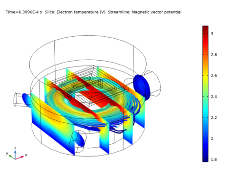
In the Settings window for Streamline, click Replace Expression in the upper-right corner of the Expression section. From the menu, choose Component 1 (comp1)>Magnetic Fields>Magnetic>Ax,Ay,Az - Magnetic vector potential.
3
Locate the Data section. From the Dataset list, choose Study 1/Solution 1 (1) (sol1).
4
Locate the Streamline Positioning section. From the Positioning list, choose Starting-point controlled.
5
From the Entry method list, choose Coordinates.
6
In the x text field, type range(-0.12,0.02,0.12).
7
In the y text field, type -0.12.
8
In the z text field, type -0.05.
9
Locate the Coloring and Style section. Find the Line style subsection. From the Type list, choose Tube.
Color Expression 1
1
Right-click Streamline 1 and choose Color Expression.
2
In the Settings window for Color Expression, click Replace Expression in the upper-right corner of the Expression section. From the menu, choose Component 1 (comp1)>Magnetic Fields>Electric>mf.normE - Electric field norm - V/m.
3
Locate the Coloring and Style section. Clear the Color legend check box.
4
In the Electron Temperature (plas) toolbar, click  Plot.