PDF

Slurry Transport
Introduction
The Pipe Flow interface allows you to simulate non-Newtonian fluids flowing in pipes. You can easily switch between Newtonian and non-Newtonian fluid models using a Fluid Model property setting.
This example models a coal slurry being transported in a pipe system where the pipe diameter changes in different sections. The slurry behaves as a non-Newtonian fluid described by the power law model. Results provide the flow rate in different sections of the piping and the total pressure drop across the system.
Model Definition
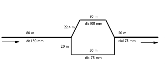
A coal slurry enters a 150 mm diameter pipe at a flow rate of 3.4 m3/min. The main pipe branches of into two loops, where the pipe diameter is 100 mm in the upper loop and 75 mm in the lower loop. The branches then rejoin in a single pipe that has a diameter of 175 mm.
Figure 1: A non-Newtonian coal slurry is transported in a system with two pipe loops.
The slurry properties are summarized below:
The mass conservation and momentum equations below describe the stationary flow of a fluid in a horizontal pipe:
(1)
(2)
The pressure losses due to pipe friction is a function of the Darcy friction factor, fD, that will be different depending upon whether the fluid is Newtonian or non-Newtonian.
The present example treats a Power-law fluid, where the apparent viscosity is related to the shear rate as
(3)
Above, where m and n are two empirical curve fitting parameters known as the fluid consistency coefficient and the flow behavior index, respectively.
In the laminar regime the friction factor for power law fluids is calculated by the Stokes equation using the modified Reynolds number proposed by Metzner and Reed (Ref. 1):
(4)
(5)
For the turbulent regime the friction model proposed by Irvine (Ref. 2) is available:
(6)
where
(7)
The Pipe Flow interface calculates a critical Reynolds number (Ref. 3) internally, which serves as a criterion for the transition between laminar and turbulent flow
(8)
If the Irvine friction model is selected and ReMR < Recrit, then the friction factor is evaluated using Equation 4. Nevertheless, it is always good practice to evaluate the Reynolds number in a pipe flow simulation to confirm that the selected friction model applies.
The friction model is specified in the Pipe Properties feature. It is possible set up multiple Pipe Properties features, and if needed assign different friction models to different parts of a pipe system.
Results and Discussion
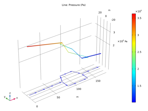
Figure 2 shows the calculated pressure in the pipe system. The total pressure drop is around 2.7·105 Pa.
Figure 2: Pipe pressure as function of position in the pipe system.
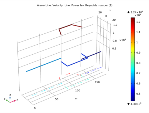
The flow rate is evaluated to 2.48 m3/min in the upper pipe loop and to 0.92 m3/min in the lower loop. Figure 3 shows a plot of ReMR in the different pipe sections, that can be used to find if the flow is laminar or turbulent. Since ReMR > Recrit, calculated to 2434 from Equation 8, it can be concluded that the flow is turbulent everywhere.
Figure 3: The Reynolds number indicates turbulent conditions in the entire pipe network.
References
1. A.B. Metzner and J.C. Reed, AICHE Journal, vol. 1, p. 434, 1955.
2. T.F. Irvine, Chem. Eng. Commun., vol. 65, p. 39, 1988.
3. N.W. Ryan and M.M. Johnson, AICHE Journal, vol. 5, p. 433, 1959.
Application Library path: Pipe_Flow_Module/Tutorials/slurry_transport
Modeling Instructions
From the File menu, choose New.
New
In the New window, click  Model Wizard.
Model Wizard
1
In the Model Wizard window, click  2D.
2
In the Select Physics tree, select Fluid Flow>Single-Phase Flow>Pipe Flow (pfl).
3
Click Add.
4
Click  Study.
5
In the Select Study tree, select General Studies>Stationary.
6
Global Definitions
Parameters 1
1
In the Model Builder window, under Global Definitions click Parameters 1.
2
In the Settings window for Parameters, locate the Parameters section.
3
Geometry 1
Polygon 1 (pol1)
1
In the Geometry toolbar, click  Polygon.
2
In the Settings window for Polygon, locate the Object Type section.
3
From the Type list, choose Open curve.
4
Locate the Coordinates section. From the Data source list, choose Vectors.
5
In the x text field, type 0 80 80 90 90 120 120 130 130 180 .
6
In the y text field, type 0 0 0 20 20 20 20 0 0 0.
Polygon 2 (pol2)
1
In the Geometry toolbar, click  Polygon.
2
In the Settings window for Polygon, locate the Object Type section.
3
From the Type list, choose Open curve.
4
Locate the Coordinates section. From the Data source list, choose Vectors.
5
In the x text field, type 80 80 80 130 130 130.
6
In the y text field, type 0 -20 -20 -20 -20 0.
7
Click  Build All Objects.
Pipe Flow (pfl)
1
In the Model Builder window, under Component 1 (comp1) click Pipe Flow (pfl).
2
In the Settings window for Pipe Flow, locate the Fluid Model section.
3
From the Fluid model list, choose Power law.
Fluid Properties 1
1
In the Model Builder window, under Component 1 (comp1)>Pipe Flow (pfl) click Fluid Properties 1.
2
In the Settings window for Fluid Properties, locate the Fluid Properties section.
3
In the m text field, type 1.4.
4
In the n text field, type 0.4.
Pipe Properties 1
1
In the Model Builder window, click Pipe Properties 1.
2
In the Settings window for Pipe Properties, locate the Pipe Shape section.
3
4
In the di text field, type d1.
Inlet 1
1
In the Physics toolbar, click  Points and choose Inlet.
2
3
In the Settings window for Inlet, locate the Inlet Specification section.
4
From the Specification list, choose Volumetric flow rate.
5
In the qv,0 text field, type Qv0.
Pipe Properties 2
1
In the Physics toolbar, click  Boundaries and choose Pipe Properties.
2
3
In the Settings window for Pipe Properties, locate the Pipe Shape section.
4
5
In the di text field, type d2.
Pipe Properties 3
1
In the Physics toolbar, click  Boundaries and choose Pipe Properties.
2
3
In the Settings window for Pipe Properties, locate the Pipe Shape section.
4
5
In the di text field, type d3.
Pipe Properties 4
1
In the Physics toolbar, click  Boundaries and choose Pipe Properties.
2
3
In the Settings window for Pipe Properties, locate the Pipe Shape section.
4
5
In the di text field, type d4.
Study 1
In the Home toolbar, click  Compute.
Results
Height Expression 1
1
In the Model Builder window, expand the Pressure (pfl) node.
2
Right-click Line 1 and choose Height Expression.
3
In the Settings window for Height Expression, locate the Expression section.
4
From the Height data list, choose Expression.
5
Click Replace Expression in the upper-right corner of the Expression section. From the menu, choose Component 1 (comp1)>Pipe Flow>pfl.ptot - Total pressure - Pa.
Arrow Line 1
1
In the Model Builder window, right-click Pressure (pfl) and choose Arrow Line.
2
In the Settings window for Arrow Line, click to expand the Title section.
3
From the Title type list, choose None.
4
Locate the Coloring and Style section. From the Arrow length list, choose Normalized.
5
From the Arrow base list, choose Center.
6
Select the Scale factor check box.
7
8
Locate the Arrow Positioning section. In the Number of arrows text field, type 14.
9
Locate the Coloring and Style section. From the Color list, choose Blue.
10
In the Pressure (pfl) toolbar, click  Plot.
The plot should like look that shown in Figure 2.
Velocity (pfl)
To reproduce Figure 3 do as follows.
Line 1
1
In the Model Builder window, right-click Velocity (pfl) and choose Line.
2
In the Settings window for Line, click Replace Expression in the upper-right corner of the Expression section. From the menu, choose Component 1 (comp1)>Pipe Flow>pfl.ReMR - Power law Reynolds number.
3
Locate the Coloring and Style section. From the Line type list, choose Tube.
Height Expression 1
Right-click Line 1 and choose Height Expression.
Color Expression 1
1
In the Model Builder window, expand the Arrow Line 1 node, then click Color Expression 1.
2
In the Settings window for Color Expression, locate the Coloring and Style section.
3
Clear the Color legend check box.
Velocity (pfl)
1
In the Model Builder window, click Velocity (pfl).
2
In the Settings window for 2D Plot Group, locate the Plot Settings section.
3
Clear the Plot dataset edges check box.
4
In the Velocity (pfl) toolbar, click  Plot.
5
Locate the Color Legend section. Select the Show maximum and minimum values check box.
6
Select the Show units check box.
Line 1
1
In the Model Builder window, click Line 1.
2
In the Settings window for Line, click to expand the Quality section.
3
From the Smoothing list, choose Inside geometry domains.
4
In the Velocity (pfl) toolbar, click  Plot.
Point Evaluation 1
1
In the Results toolbar, click  Point Evaluation.
You can evaluate the volumetric flow rate for the upper and lower loops:
2
3
In the Settings window for Point Evaluation, locate the Expressions section.
4
5
Click  Evaluate.