PDF

Organ Pipe Design
Introduction
In this model, an organ flue pipe is designed and analyzed using a pipe acoustics model. Because it is a 1D model, it is fast to solve but still retains most of the relevant physical parameters when designing an organ pipe. The model includes the elastic properties of the organ pipe walls, the end impedance properties at the open pipe end, and the possibility to add a small background airflow inside the pipe. In this model, the pipe is driven at 440 Hz which is the A4 note (or a’).
A sketch of an organ pipe is shown in Figure 1. An airflow is pushed in at the bottom of the organ pipe and out via the mouth. At the mouth, an air jet strikes the sharp upper lip and this sets the air into vibration. The vibrations resonate with the organ pipe body to create the note of the pipe. In an open pipe, like the one sketched here, the fundamental tone corresponds to a half wave resonance in the pipe. The harmonics are then multiples of this frequency.
Figure 1: Sketch of an organ pipe including the mouth and the pipe body.
Note: This application requires the Acoustics Module or the Pipe Flow Module.
The timbre of the organ pipe depends on the combination of the fundamental tone and all the harmonics. This depends on the shape of the pipe (the length and diameter) as well as on the elastic properties of the pipe walls and their thickness. Moreover, a small residual airflow in the pipe u0, may alter the natural frequencies slightly (this effect is not modeled here). Changing any of these parameters influences not only the natural frequencies of the organ pipe, but also the damping and Q value of the corresponding frequency response resonance peaks. This in turn yields a different timbre.
Model Definition
The organ pipe geometry is defined in terms of its length L, inner pipe diameter d, wall thickness dw (see Figure 1), and cross-section shape (here circular). Only the length is used when drawing the pipe geometry as a straight line segment. The inner radius, wall thickness, and pipe shape are parameters entering the governing equations. The elastic properties of the pipe wall are Young’s modulus Ew and Poisson’s ratio νw. The model parameters are given in the table below.
Lguess
c0/(2 f)
dw
Ew
109 Pa
νw
c0
ka
hmin
c0/3000 Hz/20
The open end of the pipe is modeled by adding an end impedance property. This is an engineering relation for the case of a pipe of circular cross section ending in free space (an unflanged pipe).
Results and Discussion
The frequency response of the pipe is obtained by plotting the sound pressure level Lp at the open pipe end,
where pref is the reference pressure for air, 20 μPa, and * is the complex conjugate.
The frequency response around the first resonance frequency if plotted in Figure 2 for several values of the pipe diameter. Changing the pipe diameter clearly shifts the resonance frequency but also changes the damping and Q value, that is, the width of the peak. Hence this is an important factor when designing organ pipes.
Figure 2: Resonance peak of the fundamental frequency at 440 Hz for different inner pipe diameters.
The response for different values of the pipe wall width is plotted in Figure 3. Here it is also seen that changing the pipe wall width (in general any of the pipe wall properties) changes the resonance slightly. This is because the elastic properties of the pipe wall have influence on the effective compressibility of the system in a given cross section. This in turn changes the effective speed of sound in the pipe and thus the resonance. The value of Young’s modulus in this example model was chosen to demonstrate this effect. A typical circular organ pipe is however made of a tin-lead alloy, which has a much higher value of Young’s modulus.
In the final plot in Figure 4, the parameter values giving a fundamental resonance at 440 Hz are selected (see the parameters list) and the response is plotted for frequencies from 100 Hz to 3000 Hz. The plot shows the fundamental resonance at 440 Hz as well as the following five resonance frequencies of the organ pipe. The shape of this curve is related to the timbre of the pipe.
Figure 3: Resonance peak of the fundamental frequency at 440 Hz for different pipe wall thickness.
Figure 4: Resonance peaks of the six first natural frequencies of the pipe from 100 to 3000 Hz.
Application Library path: Pipe_Flow_Module/Pipe_Acoustics/organ_pipe_design
Modeling Instructions
From the File menu, choose New.
New
In the New window, click  Model Wizard.
Model Wizard
1
In the Model Wizard window, click  3D.
2
In the Select Physics tree, select Acoustics>Pipe Acoustics>Pipe Acoustics, Frequency Domain (pafd).
3
Click Add.
4
Click  Study.
5
In the Select Study tree, select General Studies>Frequency Domain.
6
Global Definitions
Parameters 1
1
In the Model Builder window, under Global Definitions click Parameters 1.
2
In the Settings window for Parameters, locate the Parameters section.
3
Click  Load from File.
4
Geometry 1
Polygon 1 (pol1)
1
In the Geometry toolbar, click  More Primitives and choose Polygon.
2
In the Settings window for Polygon, locate the Coordinates section.
3
4
Click  Build All Objects.
Add Material
1
In the Home toolbar, click  Add Material to open the Add Material window.
2
Go to the Add Material window.
3
4
Click Add to Component in the window toolbar.
5
In the Home toolbar, click  Add Material to close the Add Material window.
Pipe Acoustics, Frequency Domain (pafd)
Set the cross-section shape of the organ pipe and the elastic properties of the pipe walls.
Fluid Properties 1
1
In the Model Builder window, under Component 1 (comp1)>Pipe Acoustics, Frequency Domain (pafd) click Fluid Properties 1.
2
In the Settings window for Fluid Properties, locate the Model Input section.
3
In the T0 text field, type T0.
4
In the p0 text field, type p0.
Pipe Properties 1
1
In the Model Builder window, click Pipe Properties 1.
2
In the Settings window for Pipe Properties, locate the Pipe Shape section.
3
4
In the di text field, type d.
5
Locate the Pipe Model section. From the Pipe model list, choose Anchored at one end.
6
From the E list, choose User defined. In the associated text field, type Ew.
7
From the ν list, choose User defined. In the associated text field, type nuw.
8
In the Δw text field, type dw.
End Impedance 1
At the open end, the organ pipe is sitting in free air. Use the Unflanged pipe, circular end impedance to get the correct acoustic behavior here. Note that a low ka limit version also exists but this one is only valid for k·a 1 . In this model k·a0.24 as seen in the parameters list.
1
In the Physics toolbar, click  Points and choose End Impedance.
2
3
In the Settings window for End Impedance, locate the End Impedance section.
4
From the Impedance model list, choose Unflanged pipe, circular.
Pressure 1
1
In the Physics toolbar, click  Points and choose Pressure.
2
3
In the Settings window for Pressure, locate the Pressure section.
4
In the pin text field, type 1.
Mesh 1
Edge 1
1
In the Mesh toolbar, click  Boundary and choose Edge.
2
Size
1
In the Model Builder window, click Size.
2
In the Settings window for Size, locate the Element Size section.
3
Click the Custom button.
4
Locate the Element Size Parameters section. In the Maximum element size text field, type h_min.
5
In the Minimum element size text field, type h_min/2.
6
Click  Build All.
Study 1
Step 1: Frequency Domain
1
In the Model Builder window, under Study 1 click Step 1: Frequency Domain.
2
In the Settings window for Frequency Domain, locate the Study Settings section.
3
In the Frequencies text field, type range(f_est-30,0.5,f_est+30).
Here the variable f_est corresponds to the estimated resonance frequency of the pipe taking the end correction into account. For narrow pipes the calculated resonance f_est is close to the ideal A4 (or a’) note of f = 440 Hz.
Parametric Sweep
The sweep over the pipe diameter is done using a Parametric Sweep.
1
In the Study toolbar, click  Parametric Sweep.
2
In the Settings window for Parametric Sweep, locate the Study Settings section.
3
4
5
In the Model Builder window, click Study 1.
6
In the Settings window for Study, type Study 1 - Inner Pipe Diameter Sweep in the Label text field.
7
In the Study toolbar, click  Compute.
Add Study
1
In the Study toolbar, click  Add Study to open the Add Study window.
2
Go to the Add Study window.
3
Find the Studies subsection. In the Select Study tree, select General Studies>Frequency Domain.
4
Click Add Study in the window toolbar.
5
In the Study toolbar, click  Add Study to close the Add Study window.
Study 2
Step 1: Frequency Domain
1
In the Settings window for Frequency Domain, locate the Study Settings section.
2
In the Frequencies text field, type range(f_est-30,0.5,f_est+30).
3
Click to expand the Study Extensions section. Select the Auxiliary sweep check box.
4
5
6
In the Model Builder window, click Study 2.
7
In the Settings window for Study, type Study 2 - Pipe Wall Thickness Sweep in the Label text field.
8
Locate the Study Settings section. Clear the Generate default plots check box.
9
In the Study toolbar, click  Compute.
Add Study
1
In the Study toolbar, click  Add Study to open the Add Study window.
2
Go to the Add Study window.
3
Find the Studies subsection. In the Select Study tree, select General Studies>Frequency Domain.
4
Click Add Study in the window toolbar.
5
In the Study toolbar, click  Add Study to close the Add Study window.
Study 3
Step 1: Frequency Domain
1
In the Settings window for Frequency Domain, locate the Study Settings section.
2
In the Frequencies text field, type range(100,10,3000).
3
In the Model Builder window, click Study 3.
4
In the Settings window for Study, type Study 3 - Extended Frequency Sweep in the Label text field.
5
Locate the Study Settings section. Clear the Generate default plots check box.
6
In the Study toolbar, click  Compute.
Results
Acoustic Pressure (pafd)
The first two figures show the pressure distribution and the velocity field in the pipe section as line plots in 3D. You can select different parameter values and frequencies and evaluate the plots to study the pressure distribution in the pipe.
Next, create three plots that show the frequency response of the organ pipe. This is here the sound pressure level evaluated at the open end of the of the pipe for three different cases. The first shows the fundamental resonance and how it depends on the inner tube diameter. The next shows the dependency on the tube wall thickness. The final plot shows the solution for a larger frequency range including the six first resonance frequencies.
Response: Different Pipe Diameters
1
In the Home toolbar, click  Add Plot Group and choose 1D Plot Group.
2
In the Settings window for 1D Plot Group, locate the Data section.
3
From the Dataset list, choose Study 1 - Inner Pipe Diameter Sweep/Parametric Solutions 1 (sol2).
4
In the Label text field, type Response: Different Pipe Diameters.
5
Click to expand the Title section. From the Title type list, choose Label.
Point Graph 1
1
Right-click Response: Different Pipe Diameters and choose Point Graph.
2
3
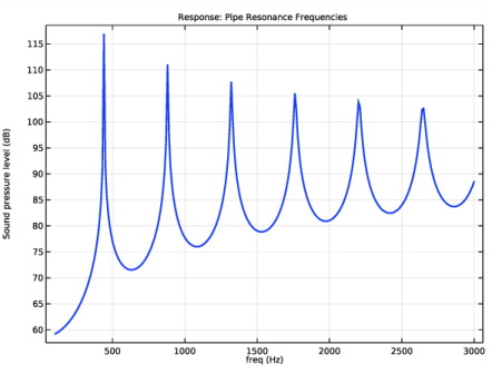
In the Settings window for Point Graph, click Replace Expression in the upper-right corner of the y-Axis Data section. From the menu, choose Component 1 (comp1)>Pipe Acoustics, Frequency Domain>Intensity and sound pressure level>pafd.Lp - Sound pressure level - dB.
4
Click to expand the Coloring and Style section. In the Width text field, type 2.
5
Click to expand the Legends section. Select the Show legends check box.
6
Find the Include subsection. Clear the Point check box.
7
In the Response: Different Pipe Diameters toolbar, click  Plot.
The figure should look like the one in Figure 2.
Response: Different Wall Thicknesses
1
In the Home toolbar, click  Add Plot Group and choose 1D Plot Group.
2
In the Settings window for 1D Plot Group, locate the Data section.
3
From the Dataset list, choose Study 2 - Pipe Wall Thickness Sweep/Solution 8 (sol8).
4
In the Label text field, type Response: Different Wall Thicknesses.
5
Locate the Title section. From the Title type list, choose Label.
Point Graph 1
1
Right-click Response: Different Wall Thicknesses and choose Point Graph.
2
3
In the Settings window for Point Graph, locate the y-Axis Data section.
4
In the Expression text field, type pafd.Lp.
5
Locate the x-Axis Data section. From the Axis source data list, choose freq.
6
Locate the Coloring and Style section. In the Width text field, type 2.
7
Locate the Legends section. Select the Show legends check box.
8
Find the Include subsection. Clear the Point check box.
9
In the Response: Different Wall Thicknesses toolbar, click  Plot.
The figure should look like the one in Figure 3.
Response: Pipe Resonance Frequencies
1
In the Home toolbar, click  Add Plot Group and choose 1D Plot Group.
2
In the Settings window for 1D Plot Group, locate the Data section.
3
From the Dataset list, choose Study 3 - Extended Frequency Sweep/Solution 9 (sol9).
4
In the Label text field, type Response: Pipe Resonance Frequencies.
5
Locate the Title section. From the Title type list, choose Label.
Point Graph 1
1
Right-click Response: Pipe Resonance Frequencies and choose Point Graph.
2
3
In the Settings window for Point Graph, locate the y-Axis Data section.
4
In the Expression text field, type pafd.Lp.
5
Locate the Coloring and Style section. In the Width text field, type 2.
6
In the Response: Pipe Resonance Frequencies toolbar, click  Plot.
The figure should look like the one in Figure 4.